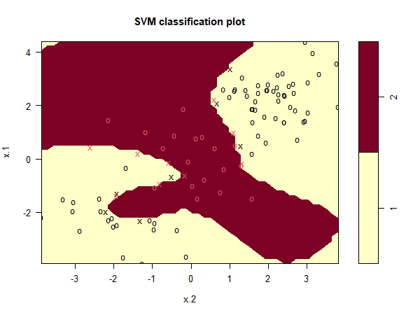
We can see from the figure that there are a fair number of training errors in this SVM fit. If we increase the value of cost, we can reduce the number of training errors. However, this comes at the price of a more irregular decision boundary that seems to be at risk of overfitting the data.

svmfit = svm(y ~ ., data = dat[train,], kernel = "radial", gamma = 1, cost = 1e5)
plot(svmfit, dat[train,])

Questions

Below three models are defined with different values (0.01, 1 and 10000) for the cost parameter.

• Calculate both the training and test accuracy of all three models to gain insights on overfitting and underfitting. Store the accuracies in train.acc1, train.acc2, train.acc3, test.acc1, test.acc2 and test.acc3 for all three models respectively.

MC1: Which of these statements are true?
1) Model 3 has a perfect training accuracy and thus is the best performing model
2) Since model 1 has a low training accuracy and low test accuracy, we can say the model is overfitting on the training data
3) Model 2 generalizes the best to unseen data compared to the other models

You can easily calculate the accuracy by comparing the predicted values with the actual values and taking the mean of that boolean vector: mean(predict(svmfit, dat[train,]) == dat[train,"y"])

---

Assume that:

• The e1071 library has been loaded