T-SNE
In this exercise, we’ll be visualizing word embeddings using t-SNE, a technique for dimensionality reduction that is particularly well-suited for visualizing high-dimensional datasets (like embeddings). It’s comparable to PCA.
We’ll be working with the word_vectors we created in the previous exercise.
Preparing the Data
First, let’s create a vector of words to keep before applying t-SNE. We want to remove stop words, which should ideally be filtered out at the beginning, but it’s always good to double-check.
keep_words <- setdiff(rownames(word_vectors), stopwords())
Next, we’ll keep the words in a vector.
word_vec <- word_vectors[keep_words,]
Then, we’ll prepare a data frame for training.
train_df <- data.frame(word_vec) %>%
  rownames_to_column("word")
Training t-SNE for Visualization
Now, we can train t-SNE for visualization.
tsne <- Rtsne(train_df[,-1],
              dims = 2, perplexity = 30,
              verbose=TRUE, max_iter = 500)
Perplexity controls how many nearest neighbors are included.
The default value is equal to 30.
The number of iterations should be set high default: 1000.
Creating a Plot
Finally, we’ll create a plot.
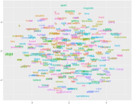
colors = rainbow(length(unique(train_df$word)))
names(colors) = unique(train_df$word)

plot_df <- data.frame(tsne$Y) %>%
  mutate(
    word = train_df$word,
    col = colors[train_df$word]) %>%
  left_join(vocab, by = c("word" = "term"))

ggplot(plot_df, aes(X1, X2, label = word, color = col)) +
  geom_text(size = 4) +
  xlab("") + ylab("") +
  theme(legend.position = "none")
The first line of code ensures that every unique words gets another color.
T-SNE maps high dimensional data such as word embedding into a lower dimension in such that the distance between two words roughly describe the similarity. The closer the observations are in the embedding space, the more similar they are. Can you spot any clusters?
Multiple Choice
The plot below is one from the hotel reviews. Type the correct answer (1, 2 or 3) into the environment.
- The perplexity can be the same as that of the example with product reviews.
- The perplexity can be lower as that of the example with product reviews.
- The perplexity can be higher as that of the example with product reviews.
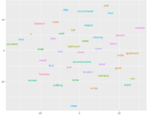
Assume that:
- The object
keep_wordscontains 374 words for the product reviews. - The object
keep_wordscontains 41 words for the hotel reviews.