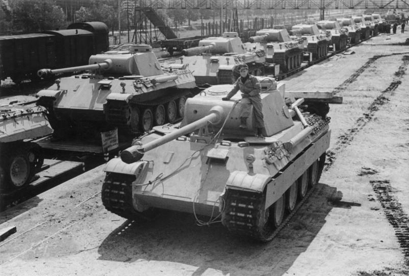
During the course of World War II, the Western Allies made sustained efforts to determine the extent of German production and approached this in two major ways: conventional intelligence gathering and statistical estimation. In many cases, statistical analysis substantially improved on conventional intelligence. This was for example the case in the estimation of Panzerkamfwagen V tank1 (better known as the Panther) production just prior to D-day2.

The allied command structure had thought the Panther tanks seen in Italy — with their high velocity, long-barreled 75 mm/L70 guns3 — were unusual heavy tanks and would only be seen in northern France in small numbers, much the same way as the Tiger I4 was seen in Tunisia. The US Army was confident that the M4 Sherman5 tank would continue to perform well, as it had versus the Panzer III6 and Panzer IV7 tanks in North Africa and Sicily. However, shortly before D-Day, rumors indicated that large numbers of Panther tanks were being used.
To ascertain whether this was true, the Allies attempted to estimate the number of tanks being produced. To do this, they used the serial numbers on captured or destroyed tanks. The principal numbers used were gearbox numbers, as these fell in two unbroken sequences. Chassis, engine and tank wheel numbers were also used, though their use was more complicated. Various other components were used to cross-check the analysis.
According to conventional Allied intelligence estimates, the Germans were producing around 1,400 Panther tanks a month between June 1940 and September 1942. Based on statistical analysis of the serial numbers on gearboxes of captured tanks, the number was estimated to be 256 a month, which was still substantially more than had previously been suspected.
After the war, captured German production records from the ministry of Albert Speer8 showed the actual number to be 255 per month during those three years. Almost precisely what the statisticians had predicted, and less than 20 percent of the intelligence estimate. The following table shows some more details on production figures and estimates made by the Allies.
| month | statistical estimate | intelligence estimate | German records |
|---|---|---|---|
| June 1940 | 169 | 1,000 | 122 |
| June 1941 | 244 | 1,550 | 271 |
| August 1942 | 327 | 1,550 | 342 |
The statistical approach proved to be far more accurate than conventional intelligence methods, and the phrase German tank problem9 became accepted as a descriptor for this type of statistical analysis.
Assignment
Suppose German tanks are numbered sequentially $$1, 2, 3, \ldots, t$$ where $$t$$ is the total number of produced tanks that we seek to know. Also suppose that we have captured five tanks whose serial numbers are 21, 35, 42, 60 and 89. It turns out that we can use these serial numbers to make quite an accurate estimate of the total number of produced tanks $$t$$ using the following formula: \[t \approx \frac{(n + 1)m}{n} - 1\] where $$n$$ is the number of observed serial numbers (here $$n = 5$$) and $$m$$ is the largest serial number observed (here $$m = 89$$). In this example, the formula tells us that $$t = 105.8$$, so we could estimate that 106 German tanks had been produced at that time.
Input
The input contains a sequence of positive integers, each on a separate line. All numbers in the sequence are different. These numbers represent serial numbers on German tanks captured or destroyed by the Western Allies. The sequence ends with a negative integer.
Output
The output must contain the following text fragment
The number of produced tanks is estimated to be t.
where t needs to be filled up with an estimate of the number of produced tanks based on the list of serial numbers from the input and the above estimation formula. The estimate needs to be rounded to the nearest integer.
Warning
In rounding to the nearest integer you should use the default rounding behavior of Python10. After all, the "nearest" integer is not unique for half values that are equally close to their two neighboring integers above and below. Python resolves this ambiguity by always selecting the even number if there are two nearest numbers.
>>> round(1.5)
2
>>> round(2.5)
2
>>> round(3.5)
4
>>> round(4.5)
4
Example
Input:
60
21
89
42
35
-1
Output:
The number of produced tanks is estimated to be 106.Epilogue
The exact same formula has also been used in non-military contexts. For example, to estimate the number of Commodore 6411 computers built, where the result (12.5 million) matches the low-end of the estimates that can be found on the Internet.
