In order to fit regression splines in R, we use the splines library. We saw that regression splines can be fit by constructing an appropriate matrix of basis functions. The bs() function generates the entire matrix of basis functions for splines with the specified set of knots. By default, cubic splines are produced. Fitting wage to age using a regression spline is simple:

library(ISLR2)
attach(Wage)
library(splines)
fit <- lm(wage ~ bs(age, knots = c(25, 40, 60)), data = Wage)
age.grid <- seq(from = min(age), to = max(age))
pred <- predict(fit, newdata = list(age = age.grid), se = TRUE)
plot(age, wage, col = "gray")
lines(age.grid, pred$fit, lwd = 2)
lines(age.grid, pred$fit + 2 * pred$se, lty = "dashed")
lines(age.grid, pred$fit - 2 * pred$se, lty = "dashed")

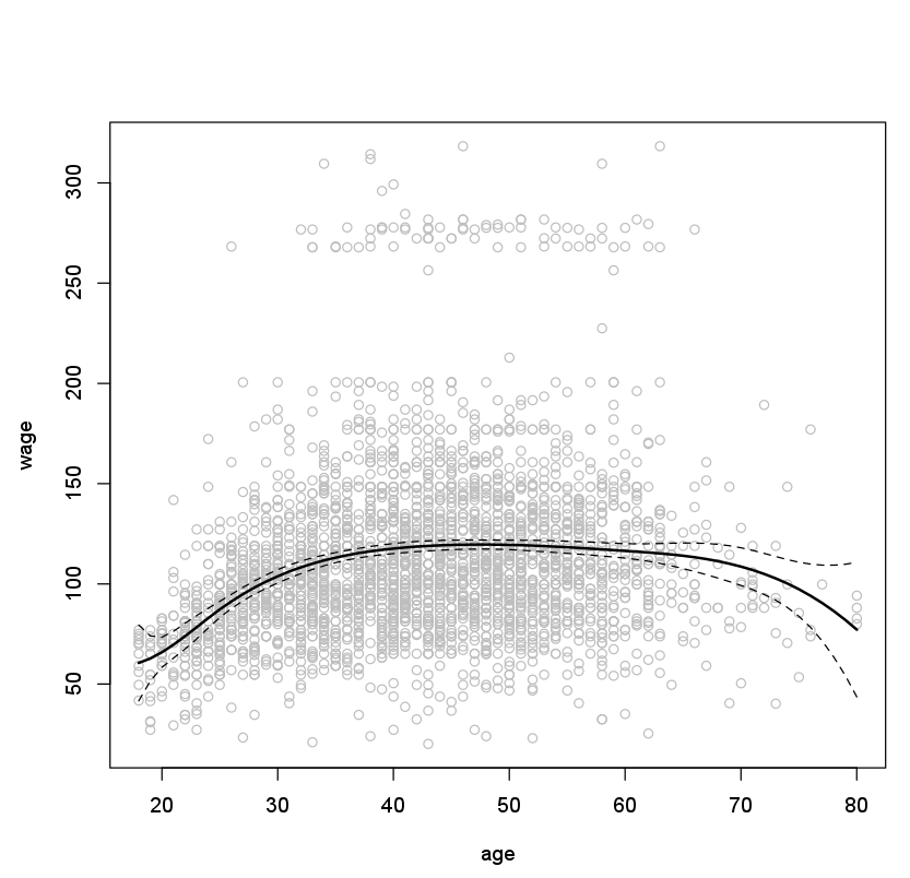
Here we have prespecified knots at ages 25, 40, and 60. This produces a spline with six basis functions. (Recall that a cubic spline with three knots has seven degrees of freedom; these degrees of freedom are used up by an intercept, plus six basis functions.) We could also use the df option to produce a spline with knots at uniform quantiles of the data.

dim(bs(age, knots = c(25, 40, 60)))
[1] 3000    6

dim(bs(age, df = 6))
[1] 3000    6

attr(bs(age, df = 6), "knots")
[1] 33.75 42.00 51.00

In this case R chooses knots at ages 33.8, 42.0, and 51.0, which correspond to the 25th, 50th, and 75th percentiles of age. The function bs() also has a degree argument, so we can fit splines of any degree, rather than the default degree of 3 (which yields a cubic spline).

Questions

• Fit a regression spline on the Boston dataset with medv as dependent variable and lstat as independent variable. The spline should be of degree-3 with two knots, at positions 10 and 20. Store the result in the variable fit.
• Calculate the predictions of medv for a series of values of lstat, ranging from 0 to 50, in steps of 1. Store the results in variable preds.
• Calculate the confidence intervals with z-value 2.0. Store the results in variable se.bands.
• MC1: Inspect the dimensions of the basis function matrix, how many basis functions and degrees of freedom do we have? Recall that a cubic spline with \(K\) knots uses a total of \(4 + K\) degrees of freedom.
  • 1: 4 basis functions (+ 1 intercept) => df=5
  • 2: 5 basis functions (+ 1 intercept) => df=6
  • 3: 4 basis functions => df=4
  • 4: 5 basis functions => df=5

Assume that:

• The MASS library has been loaded
• The Boston dataset has been loaded and attached