Partial Dependence Plots
In this exercise, we will explore the concept of partial dependence plots in R.
Building the Random Forest Model
We can now create our random forest model.
rFmodel <- randomForest(
  x = BasetableTRAIN,
  y = yTRAIN,
  ntree = 1000,
  importance = TRUE
)
Understanding Partial Dependence Plots
Partial dependence plots allow us to uncover the direction of the relationship between predictor and response.
The which.class=1 parameter is very important.
The default is to take the reference category to be 0 and is never what we want.
Remember that a partial dependence plot is built for every class.
partialPlot(
  x = rFmodel,
  x.var = "Recency",
  pred.data = BasetableTRAIN,
  which.class = "1"
)
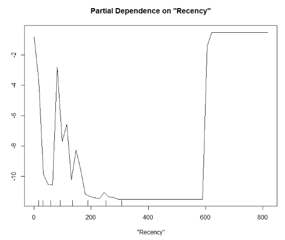
From the partial dependence plot, it can be concluded that a small recency results in a higher propensity to have a 1. Note that there is some discussion on whether to use the train or the test set. Both are correct, but here the training set is used as default (results can differ on test set).
partialPlot(
  x = rFmodel,
  x.var = "TotalDiscount",
  pred.data = BasetableTRAIN,
  which.class = "1"
)
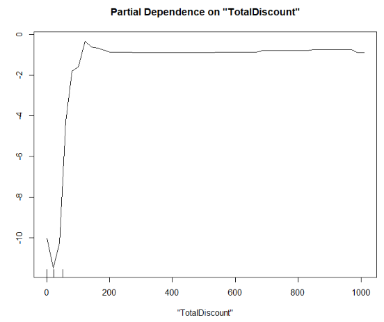
In contrast, a higher value for TotalDiscount results in a higher propensity to have a 1.
The advantage of partial dependence plots is that they display the non-linearity of the relationship.
Using the IML Package for Partial Dependence Plots
The iml package can also be used. To do so, use the FeatureEffect function.
Again, first create a Predictor object.
This function has a lot of different options, however we are only interested in partial dependence plots.
mod <- Predictor$new(
  model = rFmodel,
  data = BasetableTRAIN,
  y = yTRAIN,
  type = 'prob',
  class = 2
)
The PDP for the recency is given by the following code block.
eff <- FeatureEffect$new(mod, feature = 'Recency', method = 'pdp')
plot(eff)
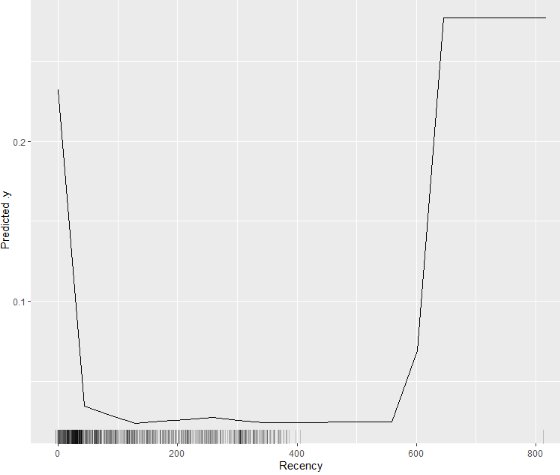
The difference with the partial function is that this function plots the actual probability.
Also note that resulting plot is again a ggplot object.
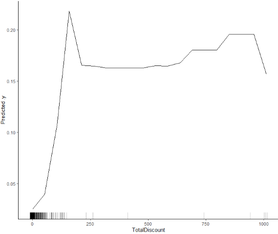
The total discount is given by the code block below.
eff <- FeatureEffect$new(mod, feature = 'TotalDiscount', method = 'pdp')
plot(eff) + theme_classic()
The joint effect of the two variables is plotted by the code block hereafter. This can take a while to run.
eff <- FeatureEffect$new(
  mod,
  feature = c('Recency', 'TotalDiscount'),
  method = 'pdp'
)
plot(eff)
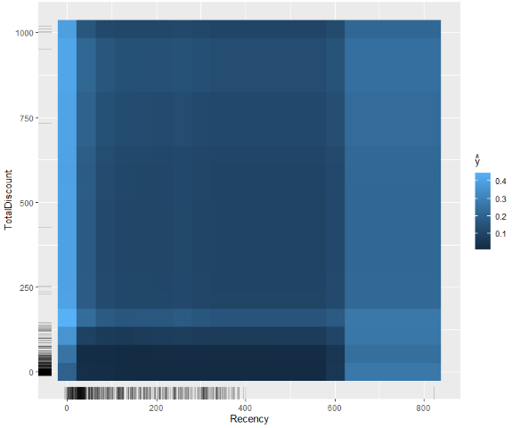
Be careful in this case with the conclusion, because the effects can be pure correlation and not causal.
Multiple choice
Consider the partial dependence plot down below. Type the number of the correct answer into the Dodona environment.
- The probability that a person is considered vaccine hesitant decreases when the number of characters in a tweet increases.
- The probability that a person is considered vaccine hesitant increases when the number of characters in a tweet increases.
- The probability that a person is considered vaccine hesitant increases when the number of characters in a tweet decreases.
- The probability that a person is considered vaccine hesitant remains the same whether the number of characters in a tweet decreases or increases.
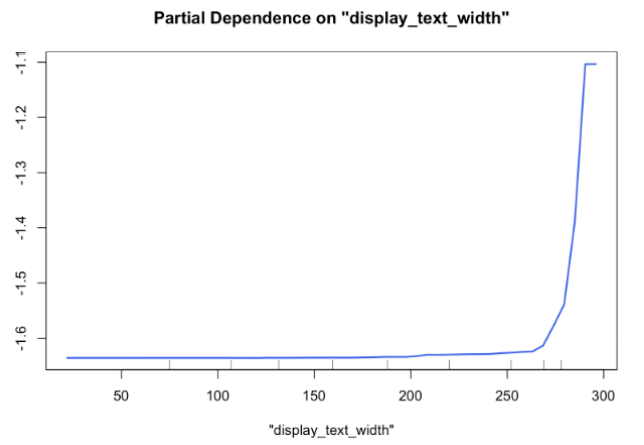
Assume that:
- The reference category is vaccine hesitant.
Display_text_witdhis the amount of characters in a tweet on Twitter.