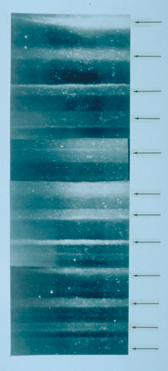
An ice core is a cylinder shaped sample that comes from an ice cap, usually from the polar regions or from a glacier. Seeing that ice caps are formed by an accumulation of yearly snow layers, they are built out of ice from different years where the under layers are older than the upper layers. Thanks to analysis of the properties of the ice and the gas composition of crystallized air bulbs that are enclosed in the ice, a climatological reconstruction can be made of the period in which the ice core was formed. Based on the concentrations and the isotopes of carbon monoxide and methane, for example, one can map out the evolution of the local temperature and the atmospheric composure.

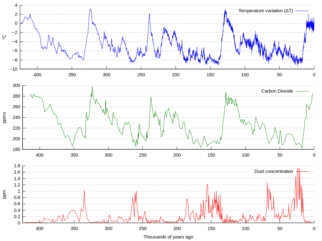
The picture above shows the evolution of temperature (blue), the concentration of carbon monoxide (green) and the amount of particles that were fixed (red) in the Vostok ice cap (Antarctica) ofer a period of the past 420.000 years. Here, a number of climatological cycles can be seen with the naked eye. However, the course of such time-series contains too much noise to immediately analyze them with a computer. This noise can be suppressed by simple mathematical techniques to level off the curves. 

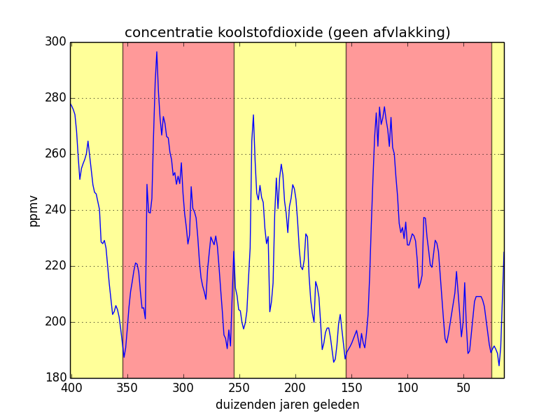
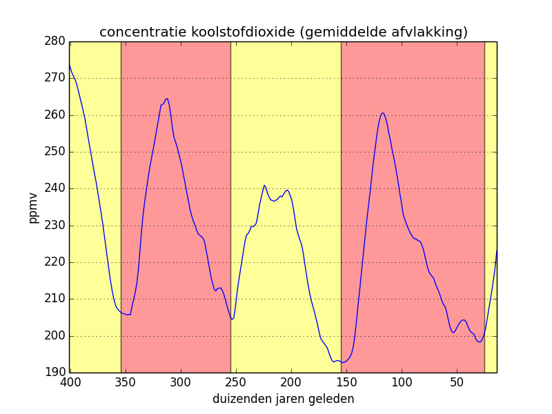
In the left-hand figure below we have copied the original values of the carbon monoxide concentration and we have indicated the climatological cycles. In the middle figure, we have applied a mean flattening to the original values and the right-hand figure is a result of a triangle flattening. In the last two cases, the periodical character of the curve is pronounced even more clearly.

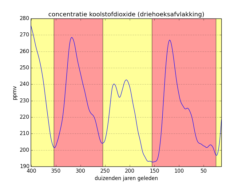
Assignment

We have determined the concentration of a certain property (e.g. the concentration of carbon monoxide) alongside consecutive points of an ice core. The values on these measurement points were bundled in a list or tuple. Your assignment is to level off these measuring values so that it is can be analyzed more easily by a computer. Work as follows:

• Say we have a sequence of $$m \in \mathbb{N}_0$$ consecutive measurements $$x_i \in \mathbb{R}$$ ($$1 \leq i \leq m$$). The weighted average $$s$$ of these measurements is obtained by linking $$w_i \in \mathbb{R}$$ ($$1 \leq i \leq m$$) to every measurement, and calculating the following \[s = \frac{\displaystyle\sum_{i=1}^m w_i x_i}{\displaystyle\sum_{i=1}^m w_i}\] For the sequence of measurements $$(4, 3, 7)$$ and the sequence of weights $$(1, 2, 1)$$ the weighted average is \[ s = \frac{4 \times 1 + 3 \times 2 + 7 \times 1}{1 + 2 + 1} = 4.25 \] Write a function weightedAverage to which two lists or tuples must be given. These arguments respectively represent a sequence of measurements $$x_i$$ ($$1 \leq i \leq m$$) and a sequence of weights $$w_i$$ ($$1 \leq i \leq m$$). If the length of the given sequences is unequal, the function must raise an AssertionError with the message sequences should have equal length. Otherwise, the function should print the weighted average $$s$$ of the given measurements, based on the weights given.

• Write a function smooth to which two lists or tuples must be given. The first argument represents a sequence of $$n \in \mathbb{N}_0$$ consecutive measurements $$x_i \in \mathbb{R}$$ ($$1 \leq i \leq n$$), and the second argument represents a sequence of $$m \in \mathbb{N}_0$$ weights $$w_i \in \mathbb{R}$$ ($$1 \leq i \leq m$$). As a result, the function should print a new list, that contains the weighted averages of all $$m$$ consecutive measurements with the given weights (see figure below). If $$n < m$$, an empty list must be printed.
  

  

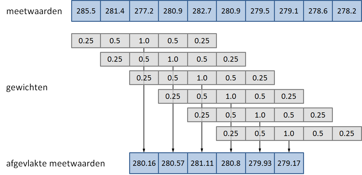
• If all weights used for flattening have the same value $$w$$ ($$w \neq 0$$), the weighted average is nothing but a normal mean of a measurement and a number of neighbouring measured values left and right of the measurement. If we use the list of weights [1, 1, 1, 1, 1], for example, 5 measurements (the measuring point and two points left and right) are averaged. This is called the mean flattening with window width $$v = 5$$. Analogously, the list with weights [1, 1, 1, 1, 1, 1, 1] is used for the mean flattening with window width $$v = 7$$. Use the function smooth to write a function smoothAverage to which an obligatory list or tuple of measurements and an optional window width $$v$$ (argument window; default value 5) must be given. The function must print a flattened list of measurements that is the result of applying the mean flattening with window width $$v$$.

• For leveling off triangles a sequence of weights is used that increases from 1 in the first part, and halfway it starts decreasing again. For example, the triangle flattening with window width $$v=5$$ uses the weights [1, 2, 3, 2, 1], the triangle flattening with window width $$v=7$$ uses the weights [1, 2, 3, 4, 3, 2, 1], and so on. Use the function smooth to write a function smoothTriangle to which an obligatory list or tuple of measurements and an optional window width $$v$$ (argument window; default value 5) must be given. If the given window width is even, the function should raise an AssertionError with the message window size must be odd value. Otherwise the function must print the flattened list of measurements that is the result after applying the triangle flattening with window width $$v$$.

Example

In the interactive session below we have rounded off the floating point numbers in order to retain a brief example. In the assignment we do not ask to round off numbers. 

>>> CO2 = [285.5, 281.4, 277.2, 280.9, 282.7]
>>> weights = [0.5, 1.0, 0.5]
>>> weightedAverage(CO2, weights )
Traceback (most recent call last):
AssertionError: sequences should have equal length
>>> weights = [0.25, 0.5, 1.0, 0.5, 0.25]
>>> weightedAverage(CO2, weights )
280.16
>>> weightedAverage((4.0, 3.0, 7.0), (1.0, 2.0, 1.0))
4.25

>>> CO2 = [285.5, 281.4, 277.2, 280.9, 282.7, 280.9, 279.5, 279.1, 278.6, 278.2]
>>> smooth(CO2, weights)
[280.16, 280.57, 281.11, 280.8, 279.93, 279.17]
>>> smoothAverage(CO2)
[281.54, 280.62, 280.24, 280.62, 280.16, 279.26]
>>> smoothAverage(CO2, window=4)
[281.25, 280.55, 280.425, 281.0, 280.55, 279.525, 278.85]
>>> smoothTriangle(CO2)
[280.489, 280.533, 280.933, 280.789, 279.978, 279.178]
>>> smoothTriangle(CO2, window=4)
Traceback (most recent call last):
AssertionError: window size must be odd value
>>> smoothTriangle(CO2, window=3)
[281.375, 279.175, 280.425, 281.8, 281.0, 279.75, 279.075, 278.625]

Resources

• Petit JR, Jouzel J, Raynaud D, Barkov NI, Barnola JM, Basile I, Bender M, Chappellaz J, Davis M, Delaygue G, Delmotte M, Kotlyakov VM, Legrand M, Lipenkov VY, Lorius C, Pépin L, Ritz C, Saltzman E, Stievenard M (1999). Climate and atmospheric history of the past 420,000 years from the Vostok ice core, Antarctica. Nature 399, 429-436. ¹

• Jouzel J, Petit JR, Souchez R, Barkov NI, Lipenkov VY, Raynaud D, Stievenard M, Vassiliev NI, Verbeke V, Vimeux F (1999). More than 200 meters of lake ice above subglacial Lake Vostok, Antarctica. Science 286(5447), 2138-2141. ²