Here we use the gbm package, and within it the gbm() function, to fit boosted regression trees to the Boston data set. We run gbm() with the option distribution="gaussian" since this is a regression problem; if it were a binary classification problem, we would use distribution="bernoulli". The argument n.trees=5000 indicates that we want 5000 trees, and the option interaction.depth=4 limits the depth of each tree.

library(gbm)
set.seed(1)
boost.boston <- gbm(medv ~ ., data = Boston[train,], distribution = "gaussian", n.trees = 5000, interaction.depth = 4)

The summary() function produces a relative influence plot and also outputs the relative influence statistics.

summary(boost.boston)
            var    rel.inf
rm           rm 43.9919329
lstat     lstat 33.1216941
crim       crim  4.2604167
dis         dis  4.0111090
nox         nox  3.4353017
black     black  2.8267554
age         age  2.6113938
ptratio ptratio  2.5403035
tax         tax  1.4565654
indus     indus  0.8008740
rad         rad  0.6546400
zn           zn  0.1446149
chas       chas  0.1443986

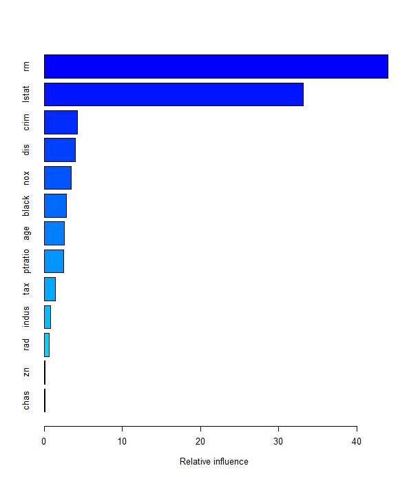
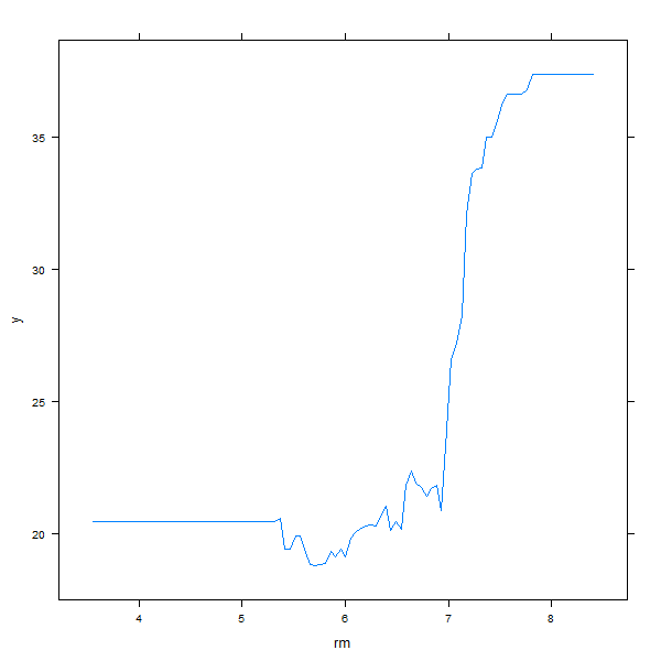
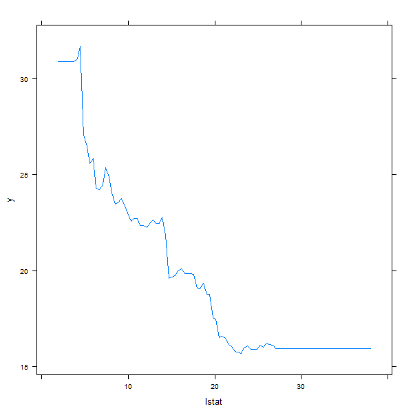
We see that lstat and rm are by far the most important variables. We can also produce partial dependence plots for these two variables. These plots illustrate the marginal effect of the selected variables on the response after integrating out the other variables. In this case, as we might expect, median house prices are increasing with rm and decreasing with lstat.

plot(boost.boston, i = "rm")
plot(boost.boston, i = "lstat")

We now use the boosted model to predict medv on the test set:

yhat.boost <- predict(boost.boston, newdata = Boston[-train,], n.trees = 5000)
mean((yhat.boost - boston.test)^2)
[1] 18.84709

The test MSE obtained is 18.85; similar to the test MSE for random forests and superior to that for bagging. If we want to, we can perform boosting with a different value of the shrinkage parameter \(\lambda\) in \(\hat f(x) \leftarrow \hat f(x) + \lambda \hat f^b(x)\). The default value is 0.1, but this is easily modified. Here we take \(\lambda = 0.2\).

boost.boston <- gbm(medv ~ ., data = Boston[train,], distribution = "gaussian", n.trees = 5000, interaction.depth = 4, shrinkage = 0.2, verbose = F)
yhat.boost <- predict(boost.boston, newdata = Boston[-train,], n.trees = 5000)
mean((yhat.boost - boston.test)^2)
[1] 18.33455

In this case, using \(\lambda = 0.2\) leads to a slightly lower test MSE than \(\lambda = 0.1\).

Questions

The Smarket data set contains the daily percentage returns for the S&P 500 stock index between 2001 and 2005. In this question we will try to predict whether a stock will go up or down (Direction) based on the its activity of the previous 5 days (Lag1, Lag2…).

library(ISLR2)
data(Smarket)

dim(Smarket)
[1] 1250    9

head(Smarket)
  Year   Lag1   Lag2   Lag3   Lag4   Lag5 Volume  Today Direction
1 2001  0.381 -0.192 -2.624 -1.055  5.010 1.1913  0.959        Up
2 2001  0.959  0.381 -0.192 -2.624 -1.055 1.2965  1.032        Up
3 2001  1.032  0.959  0.381 -0.192 -2.624 1.4112 -0.623      Down
4 2001 -0.623  1.032  0.959  0.381 -0.192 1.2760  0.614        Up
5 2001  0.614 -0.623  1.032  0.959  0.381 1.2057  0.213        Up
6 2001  0.213  0.614 -0.623  1.032  0.959 1.3491  1.392        Up

• Create a new column Target in the Smarket dataframe which has the value 1 if the stock went up and 0 if the stock went down.
• Create a training set of all the observations from 2001 to 2004 (2004 included). Store the dataframe in train.

• Create a test set of all the observations in 2005. Store the dataframe in test.

• Train a boosted classification tree on the training data with Target as the dependent variable and Lag1 to Lag5 as the independent variables and store in an object named fit.
  • For the individual classifiers use 100 decision stumps, these are decision trees with a depth of 1
  • Set the shrinkage parameter to 0.2
• Using a threshold of 0, calculate the predicted value on the test data and store them in preds. (If the model predicts a value smaller than 0, output 0, if the model predicts a value higher or equal to 0, output 1)

MC1: Does the model perform better than random guessing (accuracy higher than 50%)?

• 1: Yes
• 2: No

---

Assume that:

• The gbm and ISLR2 libraries have been loaded
• The Smarket data set has been loaded and attached