The re-sampling-based null distribution is almost identical to the theoretical null distribution, which is displayed in red.

Finally, we implement the plug-in re-sampling FDR approach outlined in Algorithm 13.4. Depending on the speed of your computer, calculating the FDR for all 2,308 genes in the Khan dataset may take a while. Hence, we will illustrate the approach on a random subset of 100 genes. For each gene, we first compute the observed test statistic, and then produce 10,000 re-sampled test statistics. This may take a few minutes to run. If you are in a rush, then you could set B equal to a smaller value (e.g. B = 500).

m <- 100
set.seed(1)
index <- sample(ncol(x1), m)
Ts <- rep(NA, m)
Ts.star <- matrix(NA, ncol = m, nrow = B)
for (j in 1:m) {
  k <- index[j]
  Ts[j] <- t.test(x1[, k], x2[, k], var.equal = TRUE)$statistic
  for (b in 1:B) {
    dat <- sample(c(x1[, k], x2[, k]))
    Ts.star[b, j] <- t.test(dat[1:n1], dat[(n1 + 1):(n1 + n2)], var.equal = TRUE)$statistic
  }
}

Next, we compute the number of rejected null hypotheses \(R\), the estimated number of false positives \(\widehat V\) , and the estimated FDR, for a range of threshold values \(c\) in Algorithm 13.4. The threshold values are chosen using the absolute values of the test statistics from the 100 genes.

cs <- sort(abs(Ts))
FDRs <- Rs <- Vs <- rep(NA, m)
for (j in 1:m) {
  R <- sum(abs(Ts) >= cs[j])
  V <- sum(abs(Ts.star) >= cs[j]) / B
  Rs[j] <- R
  Vs[j] <- V
  FDRs[j] <- V / R
}

Now, for any given FDR, we can find the genes that will be rejected. For example, with the FDR controlled at 0.1, we reject 15 of the 100 null hypotheses. On average, we would expect about one or two of these genes (i.e. 10% of 15) to be false discoveries. At an FDR of 0.2, we can reject the null hypothesis for 28 genes, of which we expect around six to be false discoveries. The variable index is needed here since we restricted our analysis to just 100 randomly-selected genes.

> max(Rs[FDRs <= .1])
[1] 15
> sort(index[abs(Ts) >= min(cs[FDRs < .1])])
 [1]   29  465  501  554  573  729  733 1301 1317 1640 1646 1706 1799 1942 2159
> max(Rs[FDRs <= .2])
[1] 28
> sort(index[abs(Ts) >= min(cs[FDRs < .2])])
 [1]   29   40  287  361  369  465  501  554  573  679  729  733  990 1069 1073
[16] 1301 1317 1414 1639 1640 1646 1706 1799 1826 1942 1974 2087 2159

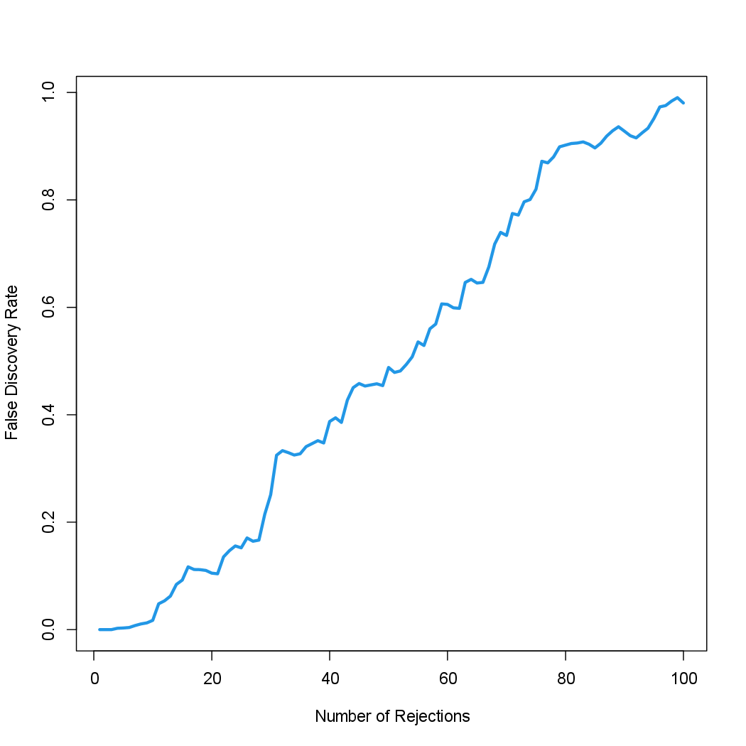
The next line generates Figure 13.11, which is similar to Figure 13.9, except that it is based on only a subset of the genes.

plot(Rs, FDRs, xlab = "Number of Rejections", type = "l", ylab = "False Discovery Rate", col = 4, lwd = 3)

As noted in the chapter, much more efficient implementations of the resampling approach to FDR calculation are available, using e.g. the samr package in R.