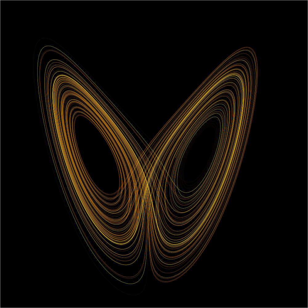
Chaos theory¹ is a field of study in mathematics, with applications in several disciplines including meteorology, physics, engineering, economics and biology. It studies the behavior of dynamical systems that are highly sensitive to initial conditions, an effect which is popularly referred to as the butterfly effect².

Small differences in initial conditions — such as those due to rounding errors in numerical computation — yield widely diverging outcomes for such dynamical systems, rendering long-term prediction impossible in general. This happens even though these systems are deterministic, meaning that their future behavior is fully determined by their initial conditions, with no random elements involved. In other words, the deterministic nature of these systems does not make them predictable.

This behavior is known as deterministic chaos, or simply chaos. The theory was summarized by Edward Lorenz³ as:

The fluttering of a butterfly's wing in Rio de Janeiro, amplified by atmospheric currents, could cause a tornado in Texas two weeks later.

— Edward Lorenz

Assignment

The following simple model for population growth might be applied to study fish in a pond, bacteria in a test tube, or any of a host of similar situations. We suppose that the population ranges from 0 (extinct) to 1 (maximum population that can be sustained).

If the population at time $$t_i$$ is $$d$$, then we suppose the population at time $$t_{i+1}$$ to be $$rd(1-d)$$, where the argument $$r$$ — known as the fecundity parameter — controls the growth rate.

Input

Three lines containing i) the initial density $$d \in \mathbb{R}$$ of a population, ii) the fecundicity parameter $$r \in \mathbb{R}$$, and iii) the number of time steps $$s \in \mathbb{N_0}$$ we want to simulate the population density (including time point $$t_0$$).

Output

$$s$$ lines containing the population density at time points $$t_0, t_1, \ldots, t_{s-1}$$.

Example

If $$r$$ has a value of around $$2$$, the population density will approach $$1 - \frac{1}{r}$$ as time progresses.

Input:

0.1
1.9
6

Output:

0.1
0.171
0.26934210000000003
0.373914173018421
0.44479449204530547
0.4692094685937818

Example

If $$r = 3$$ the population density will converge to a state where the population density alternates between two values.

Input:

0.1
3
12

Output:

0.1
0.2700000000000001
0.5913000000000002
0.7249929299999999
0.5981345443500454
0.7211088336156269
0.603332651091411
0.7179670896552621
0.6074710434816448
0.7153499244388992
0.6108732301324811
0.7131213805199696

Example

If $$r \geq 4$$ the model will behave in a chaotic way. This means that the results can change drastically when the initial conditions are slightly perturbed. See the difference in behavior between this example and the next example.

Input:

0.1
4
60

Output:

0.1
0.36000000000000004
0.9216
... (54 lines) ...
0.977464119602946
0.08811205796713474
0.32139329283172413

Example

A difference of $$0.00000000001$$ in the initial population density causes a huge difference in the population density at time point $$t_{59}$$. This is chaotic behaviour, showing that it is hard to predict population densities, because tiny pertubations cause large differences in the long run.

Input:

0.10000000001
4
60

Output:

0.10000000001
0.36000000003200006
0.9216000000358401
... (54 lines) ...
0.830632498181969
0.5627286045838009
0.9842604886678766