The rotation matrix provides the principal component loadings; each column of pr.out$rotation contains the corresponding principal component loading vector.

> pr.out$rotation
                PC1        PC2        PC3         PC4
Murder   -0.5358995  0.4181809 -0.3412327  0.64922780
Assault  -0.5831836  0.1879856 -0.2681484 -0.74340748
UrbanPop -0.2781909 -0.8728062 -0.3780158  0.13387773
Rape     -0.5434321 -0.1673186  0.8177779  0.08902432

We see that there are four distinct principal components. This is to be expected because there are in general \(min(n - 1, p)\) informative principal components in a data set with \(n\) observations and \(p\) variables.

Using the prcomp() function, we do not need to explicitly multiply the data by the principal component loading vectors in order to obtain the principal component score vectors. Rather the 50×4 matrix x has as its columns the principal component score vectors. That is, the \(k\)th column is the \(k\)th principal component score vector.

> dim(pr.out$x)
[1] 50  4

We can plot the first two principal components as follows:

biplot(pr.out, scale = FALSE)

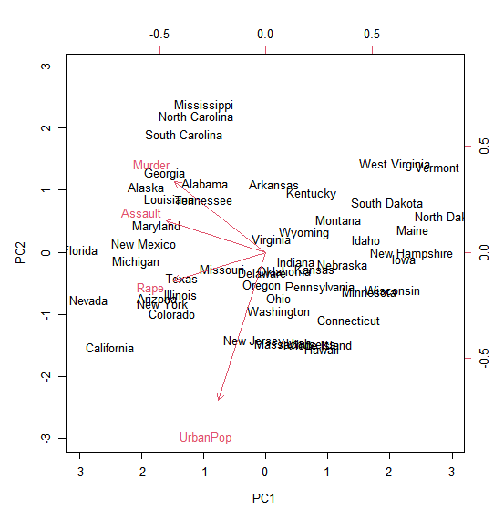
The scale=0 argument to biplot() ensures that the arrows are scaled to represent the loadings; other values for scale give slightly different biplots with different interpretations.

In the plot above, only the first two principal components are plotted. By default the function show the two most important principal components. However, you can change the choices parameter to pick other combinations of principal components. This code would give the same outcome as the plot above, since we specify the first and second principal component:

biplot(pr.out, choices = c(1, 2),scale = FALSE)

Assign TRUE or FALSE to the following statements.

Statement 1 (S1) : The arrows give us insight in the factor loadings of the different variables.

Statement 2 (S2) : The individual ‘points’, represented by the individual state names represent the principal component scores for each state.