In ggplot2 we create graphs by adding layers. Layers can define geometries, compute summary statistics, define what scales to use, or even change styles. To add layers, we use the + operator, do not use the pipe operator %>%!

In general, a line of code will look like this:

Dataframe %\>% ggplot() +
                LAYER 1 +
                LAYER 2 +
                … +
                LAYER N

Usually, the first added layer defines the geometry. We want to make a scatterplot. What geometry do we use?

Taking a quick look at the cheat sheet, we see that the function used to create plots with this geometry is geom_point.

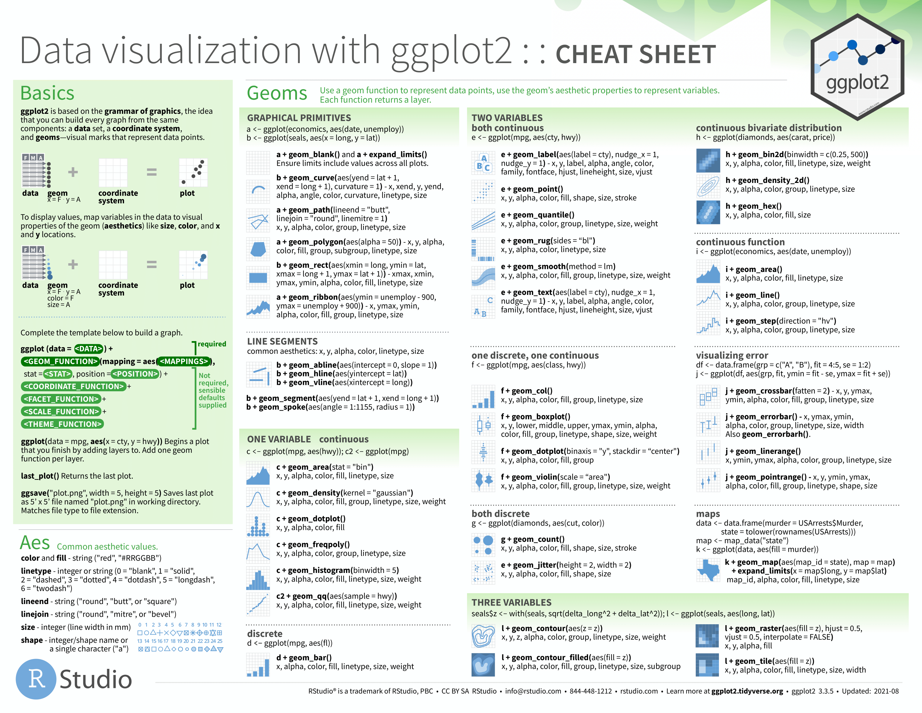
(Image courtesy of RStudio¹. CC-BY-4.0 license².)

Geometry function names follow the pattern: geom_X where X is the name of the geometry. Some examples include geom_point, geom_bar, and geom_histogram.

For geom_point to run properly we need to provide data and an aesthetics mapping. We have already connected the object p with the murders data table, and if we add the layer geom_point it defaults to using this data. To find out what mappings are expected, we read the Aesthetics section of the geom_point help file:

> Aesthetics
>
> geom_point understands the following aesthetics (required aesthetics are in bold):
>
> x
> y
> alpha
> colour
> fill
> group
> shape
> size
> stroke

and, as expected, we see that at least two arguments are required x and y.