Until now, we have been using data sets already stored as R objects. A data scientist will rarely have such luck and will have to import data into R from either a file, a database, or other sources. There are multiple ways of getting your data in (and out of) R, but we’ll discuss the three most important ones, that you will need for this course.
Loading data from within a package
This is what you have been doing until now.
Certain packages contain built-in datasets, for example the murders dataset in the dslabspackage.
You can simply load this dataset into your R environment by loading the package and then using the data()function.
library('dslabs')
data(murders)
This code should look very familiar by now.
You might observe that by just running the data() function, the dataset in the Environment pane of your RStudio seems not fully available or loaded yet.
However, as soon as you perform any action on the dataset, or as soon as you click on the dataset in the Environment pane, this ‘problem’ is solved.
Loading .RData
Another way of loading data into R is by using an .RData file.
This file can actually contain your entire R environment and can thus contain dataframes, vectors, lists, functions, …
An .RData file was constructed in R.
Consider the murders dataset that we just loaded using the first load option.
We can save this dataset that was already correctly loaded into R.
save(murders, file= 'murders_asRDataFile.RData')
Note that your file will be stored in your current working directory (more about this in one of the following sections, for now, consider this as the current location in the file structure of your PC). In order to know what your current working directory is, you can run the following function.
getwd()
You can also set your working directory yourself, for example to your Desktop, so that you will easily find your file back. Note that the directory underneath is just an example.
setwd('/home/user/Desktop/')
Now, you want to load this data again into R.
To simulate that we shut down R, first remove all objects in your environment.
You can then use the load function to load our dataset back into R.
rm(list=ls())
load('murders_asRDataFile.RData')
Reading data from a csv-file
Currently, one of the most common ways of storing and sharing data for analysis is through electronic spreadsheets. A spreadsheet stores data in rows and columns. It is basically a file version of a data frame. When saving such a table to a computer file, one needs a way to define when a new row or column ends and the other begins. This in turn defines the cells in which single values are stored.
When creating spreadsheets with text files, like the ones created with a simple text editor, a new row is defined with return and columns are separated with some predefined special character.
The most common characters are comma (,), semicolon (;), space ( ), and tab (a preset number of spaces or \t).
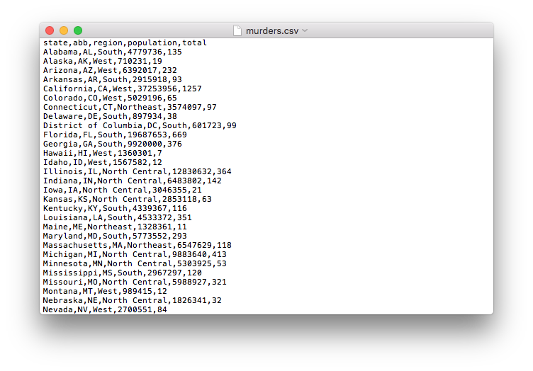
Here is an example of what a comma separated file looks like if we open it with a basic text editor (e.g. Notepad):

The first row contains column names rather than data. We call this a header, and when we read-in data from a spreadsheet it is important to know if the file has a header or not. Most reading functions assume there is a header. To know if the file has a header, it helps to look at the file before trying to read it. This can be done with a text editor (e.g. Notepad, TextEdit, Gedit).
Now, let’s create such a comma-separated values (CSV) file ourselves, so that we can load it afterwards. A csv-file is the most common type of a delimited text files. It uses a comma to separate values, hence its name.
We will make a csv-file from the murders dataset, so make sure you have this data as a data.frame in your R environment, by using one of the two methods above.
Make sure that you know your working directory (getwd()), so that you know where your csv-file will be saved.
Again, you can change your working directory with setwd() if desired.
The write.csv() function writes the murders dataframe to a csv-file that we will call murders_as_csv, with file extension .csv.
Note that we also specify the argument row.names = F because by default the row.names will be saved in the csv-file as well, however in this case, these are just the row numbers, which we don’t want to keep.
write.csv(murders, "murders_as_csv.csv", row.names = F)
Now that we created our csv-file, we are at the start point of many analyses, reading in our csv datafile.
We can use the read.csv function to read in a csv-file.
murders_read_from_csv <- read.csv("murders_as_csv.csv")
The most important optional arguments are header and sep.
These are by default set to TRUE and ,.
The header option indicates that the csv file contains a header, meaning that the first row of the file contains the column names.
The sep option refers to separator, which separates the different colums in the file.
For a standard csv-file, this is a comma indeed.
However, other options, such as tab or semicolumn are also commonly used.
You can see for yourself that the following will lead to the same result.
murders_read_from_csv_with_options <- read.csv("murders_as_csv.csv", header = T, sep = ",")