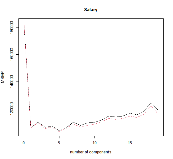
We now perform PCR on the training data and evaluate its test set performance.

                
            set.seed(1)
pcr.fit <- pcr(Salary ~ ., data = Hitters, subset = train, scale = TRUE, validation = "CV")
validationplot(pcr.fit, val.type = "MSEP")

Now we find that the lowest cross-validation error occurs when $M=5$ component are used. We compute the test $MSE$ as follows.

                
            > pcr.pred <- predict(pcr.fit, x[test,], ncomp = 5)
> mean((pcr.pred - y.test)^2)
[1] 142812

This test set $MSE$ is competitive with the results obtained using ridge regression and the lasso. However, as a result of the way PCR is implemented, the final model is more difficult to interpret because it does not perform any kind of variable selection or even directly produce coefficient estimates.

Finally, we fit PCR on the full data set, using $M=5$, the number of components identified by cross-validation.

                
            > pcr.fit <- pcr(y ~ x, scale = TRUE, ncomp = 5)
> summary(pcr.fit)
Data: 	X dimension: 263 19 
	Y dimension: 263 1
Fit method: svdpc
Number of components considered: 5
TRAINING: % variance explained
   1 comps  2 comps  3 comps  4 comps  5 comps
X    38.31    60.16    70.84    79.03    84.29
y    40.63    41.58    42.17    43.22    44.90

Questions

• Using the Boston dataset, create a PCR model using the training set provided below and store it in pcr.fit (set the ncomp parameter to 10)
• Determine the value of $M$ where the $MSE$ is minimized using the validation plot (admittedly, it is hard to see on the plot. You can also use the MSEP(pcr.fit) command to see the exact values of the $MSE$ or use the summary() function to see the $RMSE$, the minimum or $RMSE$ will be the same as the minimum of the $MSE$)
• For the optimal value of $M$, create the test predictions and store them in pcr.pred
• Finally, calculate the test $MSE$ and store it in pcr.mse

Assume that:

• The MASS and pls libraries have been loaded
• The Boston dataset has been loaded and attached