Histograms and density plots provide excellent summaries of a distribution. But can we summarize even further? We often see the average and standard deviation used as summary statistics: a two-number summary! To understand what these summaries are and why they are so widely used, we need to understand the normal distribution.
The normal distribution, also known as the bell curve and as the Gaussian distribution, is one of the most famous mathematical concepts in history. A reason for this is that approximately normal distributions occur in many situations, including gambling winnings, heights, weights, blood pressure, standardized test scores, and experimental measurement errors. There are explanations for this, but we describe these later. Here we focus on how the normal distribution helps us summarize data.
Rather than using data, the normal distribution is defined with a mathematical formula. For any interval \((a,b)\), the proportion of values in that interval can be computed using this formula:
\[\mbox{Pr}(a < x < b) = \int_a^b \frac{1}{\sqrt{2\pi}s} e^{-\frac{1}{2}\left( \frac{x-m}{s} \right)^2} \, dx\]You don’t need to memorize or understand the details of the formula. But note that it is completely defined by just two parameters: \(m\) and \(s\). The rest of the symbols in the formula represent the interval ends that we determine, \(a\) and \(b\), and known mathematical constants \(\pi\) and \(e\). These two parameters, \(m\) and \(s\), are referred to as the average (also called the mean) and the standard deviation (SD) of the distribution, respectively.
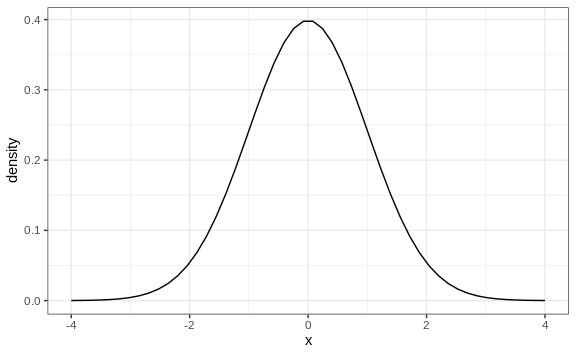
The distribution is symmetric, centered at the average, and most values (about 95%) are within 2 SDs from the average. Here is what the normal distribution looks like when the average is 0 and the SD is 1:
The fact that the distribution is defined by just two parameters implies that if a dataset is approximated by a normal distribution, all the information needed to describe the distribution can be encoded in just two numbers: the average and the standard deviation. We now define these values for an arbitrary list of numbers.
For a list of numbers contained in a vector x, the average is defined
as:
m <- sum(x) / length(x)
and the SD is defined as:
s <- sqrt(sum((x-mu)^2) / length(x))
which can be interpreted as the average distance between values and their average.
Let’s compute the values for the height for males which we will store in the object \(x\):
index <- heights$sex == "Male"
x <- heights$height[index]
The pre-built functions mean and sd (note that for reasons explained
in Section 16.2 of the Irizarry e-book, sd
divides by length(x)-1 rather than length(x)) can be used here:
m <- mean(x)
s <- sd(x)
c(average = m, sd = s)
#> average      sd
#>   69.31    3.61
Here is a plot of the smooth density and the normal distribution with mean = 69.3 and SD = 3.6 plotted as a black line with our student height smooth density in blue:
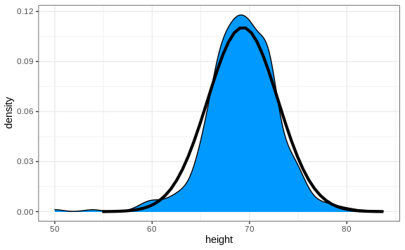
The normal distribution does appear to be quite a good approximation here. We now will see how well this approximation works at predicting the proportion of values within intervals.