Next, we add details to the model to specify the fitting algorithm. We fit the model by minimizing the cross-entropy function given by

modelnn %>% compile(loss = "categorical_crossentropy",
                    optimizer = optimizer_rmsprop(),
                    metrics = c("accuracy"))

Now we are ready to go. The final step is to supply training data, and fit the model.

system.time(
  history <- modelnn %>%
    fit(x_train, y_train, epochs = 30, batch_size = 128,
        validation_split = 0.2))
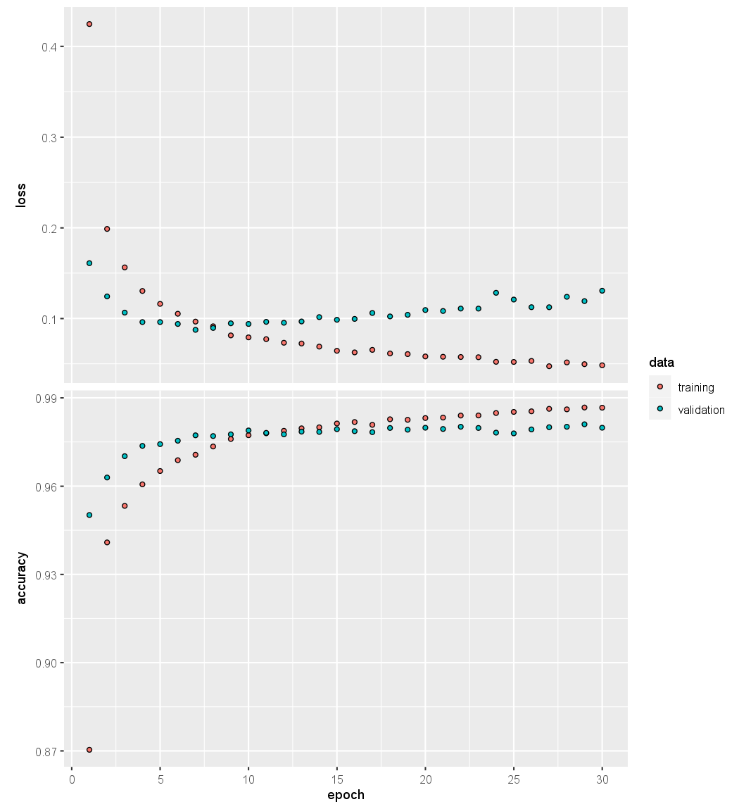
plot(history, smooth = FALSE)

We have suppressed the output here, which is a progress report on the fitting of the model, grouped by epoch. This is very useful, since on large datasets fitting can take time. Fitting this model took 144 seconds on a 2.9 GHz MacBook Pro with 4 cores and 32 GB of RAM. Here we specified a validation split of 20%, so the training is actually performed on 80% of the 60,000 observations in the training set. This is an alternative to actually supplying validation data, like we did in Section 10.9.1. See ?fit.keras.engine.training.Model for all the optional fitting arguments. SGD uses batches of 128 observations in computing the gradient, and doing the arithmetic, we see that an epoch corresponds to 375 gradient steps. The last plot() command produces a figure similar to Figure 10.18.

To obtain the test error in Table 10.1, we first write a simple function accuracy() that compares predicted and true class labels, and then use it to evaluate our predictions.

accuracy <- function(pred, truth) {
  mean(drop(as.numeric(pred)) == drop(truth))
}
modelnn %>% predict(x_test) %>% k_argmax() %>% accuracy(g_test)
[1] 0.9795

Questions

• Compile the modelnn model from the previous exercise as follows:
  • Use the categorical_crossentropy as the loss function
  • Use the optimizer_adam() as you optimizer
  • Also track the AUC as a metric (you can pass tf$keras$metrics$AUC() as an argument).
• Fit the neural network on the training data for 20 epochs and a batch size of 128. Use 20% of the training data for validation. Store the result in history.
• Visualize the loss and accuracy of the training and validation data in function of the number of epochs.
• Store the predictions on the test data of the neural network in npred.
• Store the AUC of the neural network on the test data in nauc. Use the function pROC::auc(pROC::roc(drop(response), as.numeric(drop(predictor)))), with response and predictor obtained in the previous steps.