We will now plot medv and lstat along with the least squares regression line using the plot() and abline() functions.

plot(lstat, medv)
abline(lm.fit)

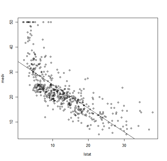
There is some evidence for non-linearity in the relationship between lstat and medv. We will explore this issue later in this lab.

The abline() function can be used to draw any line, not just the least squares regression line. To draw a line with intercept a and slope b, we type abline(a,b). Below we experiment with some additional settings for plotting lines and points. The lwd=3 command causes the width of the regression line to be increased by a factor of 3; this works for the plot() and lines() functions also.

Try-out the code below in R-Studio and see the effect of the different arguments.

abline(lm.fit, lwd = 3)
abline(lm.fit, lwd = 3, col = "red")
plot(lstat, medv, col = "red")

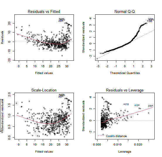
Next we examine some diagnostic plots. Four diagnostic plots are automatically produced by applying the plot() function directly to the output from lm(). In general, this command will produce one plot at a time, and hitting Enter will generate the next plot. However, it is often convenient to view all four plots together. We can achieve this by using the mfrow arugment of the par() function, which tells R to split the display screen into separate panels so that multiple plots can be viewed simultaneously. For example, par(mfrow=c(2,2)) divides the plotting region into a 2 × 2 grid of panels.

par(mfrow = c(2, 2))
plot(lm.fit)

After you have created a plot with 4 panels, it is often a good idea to set the parameters of the plot back to its default value. In this case, we want that future plots are not longer formated in a 2 x 2 grid.

par(mfrow = c(1, 1))

We can also compute the residuals from a linear regression fit using the residuals() function. The function rstudent() will return the studentized residuals, and we can use this function to plot the residuals against the fitted values.

plot(predict(lm.fit), residuals(lm.fit))
plot(predict(lm.fit), rstudent(lm.fit))

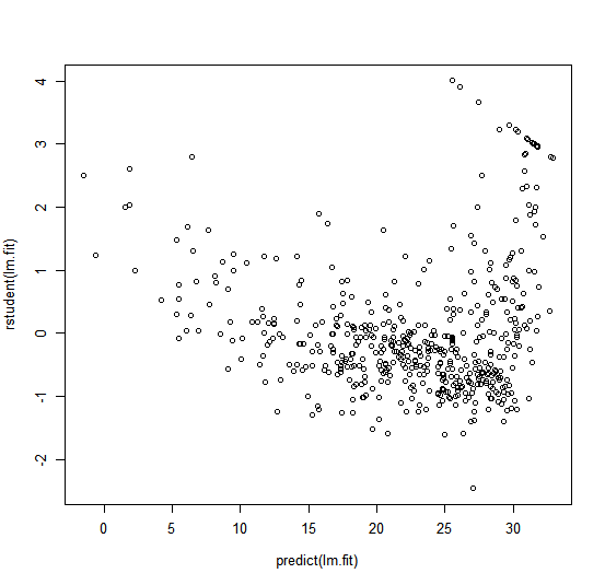
On the basis of the residual plots, there is some evidence of non-linearity. Leverage statistics can be computed for any number of predictors using the hatvalues() function.

plot(hatvalues(lm.fit))
which.max(hatvalues(lm.fit))
375

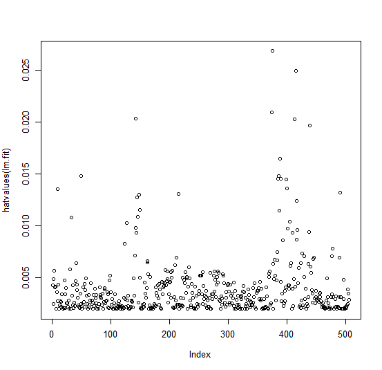
The which.max() function identifies the index of the largest element of a vector. In this case, it tells us which observation has the largest leverage statistic.