Questions

1. We now create a plot displaying \(\sqrt{\sum_{j=1}^p(\beta_j - \hat{\beta}_j^r)^2}\) for a range of values of \(r\) where \(\hat{\beta}_j^r\) is the j-th coefficient estimate for the best model containing \(r\) coefficients.

    val.errors <- rep(NA, 20)
    x_cols <- colnames(x, do.NULL = FALSE, prefix = "x.")
    for (i in 1:20) {
        coefi <- coef(regfit.full, id = i)
        val.errors[i] <- sqrt(sum((b[x_cols %in% names(coefi)] - coefi[names(coefi) %in% x_cols])^2) + sum(b[!(x_cols %in% names(coefi))])^2)
    }
    plot(val.errors, xlab = "Number of coefficients", ylab = "Error between estimated and true coefficients", pch = 19, type = "b")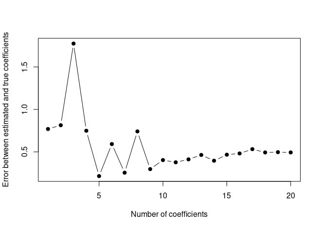
   

   

   The plot displays the errors between the estimated and the true coefficients. We can see that the model with 5 (which.min(val.errors)) variables minimizes the error between the estimated and true coefficients. However test error is minimized by the model with 15 variables (which.min(test.errors) from the previous exercise). So, a better fit of true coefficients doesn’t necessarily mean a lower test MSE!