Now consider a situation in which the two classes are linearly separable.
Then we can find a separating hyperplane using the svm() function. We
first further separate the two classes in our simulated data so that they are
linearly separable:
x[y == 1,] <- x[y == 1,] + 0.5
plot(x, col = (y + 5) / 2, pch = 19)
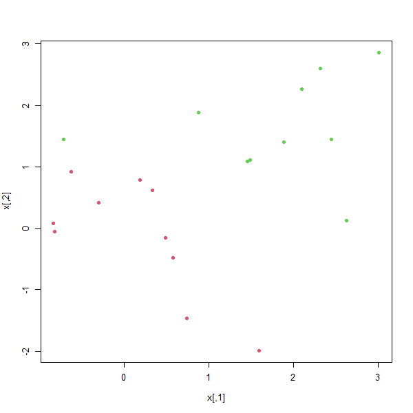
Now the observations are just barely linearly separable. We fit the support
vector classifier and plot the resulting hyperplane, using a very large value
of cost so that no training observations are misclassified.
dat <- data.frame(x = x, y = as.factor(y))
svmfit <- svm(y ~ ., data = dat, kernel = "linear", cost = 1e5)
summary(svmfit)
Call:
svm(formula = y ~ ., data = dat, kernel = "linear",
    cost = 1e+05)
Parameters:
   SVM-Type:  C-classification
 SVM-Kernel:  linear
       cost:  1e+05
Number of Support Vectors:  3
 ( 1 2 )
Number of Classes:  2
Levels:
 -1 1

plot(svmfit, dat)
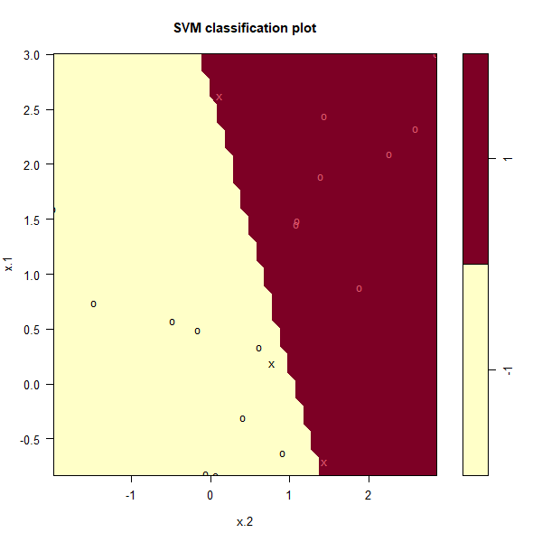
Note: The axis are swapped compared to the previous graph
No training errors were made and only three support vectors were used.
However, we can see from the figure that the margin is very narrow (because
the observations that are not support vectors, indicated as circles, are very
close to the decision boundary). It seems likely that this model will perform
poorly on test data. We now try a smaller value of cost:
svmfit <- svm(y ~ ., data = dat, kernel = "linear", cost = 1)
summary(svmfit)
plot(svmfit, dat)
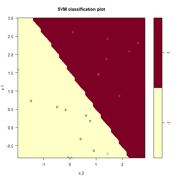
Using cost=1, we misclassify a training observation, but we also obtain
a much wider margin and make use of seven support vectors.
MC1: Which model would most likely perform better on test data
1) Model with cost = 1
2) Model with cost = 1e5