Determining Sentiment
Change the encoding and remove special characters
In the third step, we first set the encoding and remove special characters of the Facebook tweets.
Encoding(text) <- "latin1"
text <- iconv(text,'latin1', 'ascii', sub = '')
Determining the sentiment
To determine the sentiment we do not need a document-term matrix. All we need to do is
splitting the string in multiple substrings (or in other words tokenize)
and match it with the lexicon. Therefore, we will only use the
str_split function from the stringr package. Note that
str_split is again an optimized version of the
strsplit base R function.
scoretweet <- numeric(length(text))

for (i in 1:length(text)){

  #Transform text to lower case
  text <- tolower(text)

  #Split the tweet in words
  tweetsplit <- str_split(text[i]," ")[[1]]

  #Find the positions of the words in the Tweet in the dictionary
  m <- match(tweetsplit, dictionary$Word)

  #Which words are present in the dictionary?
  present <- !is.na(m)

  #Of the words that are present, select their valence
  wordvalences <- dictionary$VALENCE[m[present]]

  #Compute the mean valence of the tweet
  scoretweet[i] <- mean(wordvalences, na.rm=TRUE)

  #Handle the case when none of the words is in the dictionary
  if (is.na(scoretweet[i])) scoretweet[i] <- 0 else scoretweet[i] <- scoretweet[i]
}
Visualizing the sentiment
Let’s look at the result.
head(scoretweet)
[1] 0.7075 1.2550 1.7200 0.0000 0.7075 1.0920
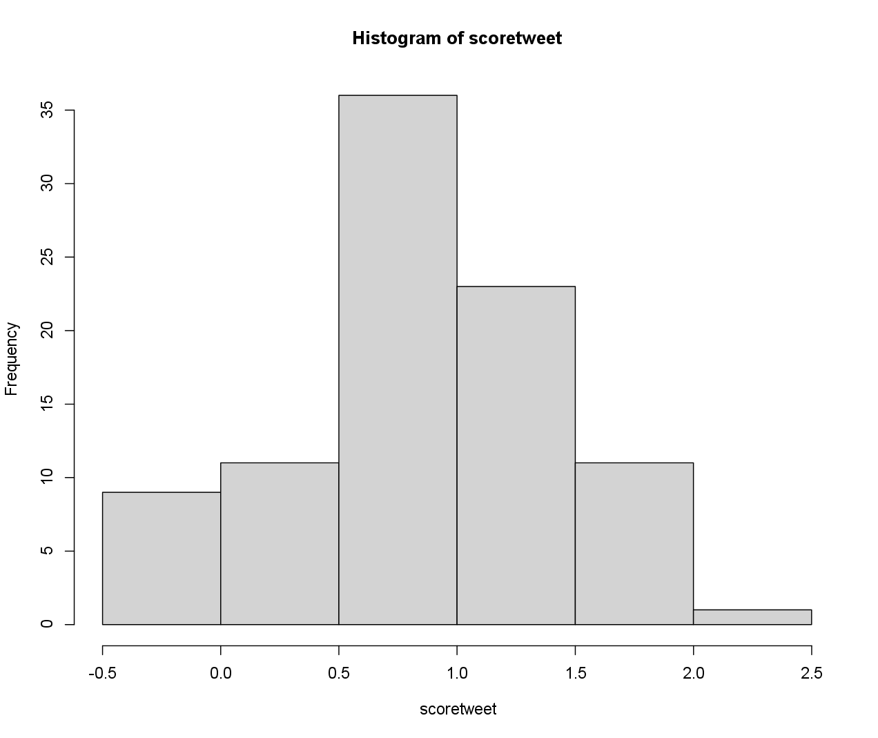
mean(scoretweet)
[1] 0.8976891
sd(scoretweet)
[1] 0.5280433
hist(scoretweet)
Let’s also look at the sentiment score per tweet.
View(bind_cols(scoretweet,text))
| ...1 | ...2 | |
|---|---|---|
| 1 | 0.707500 | don't get tired of protecting your accounts, because allot of people out there want to hack you and get access to your privacy inbox now for all hacking services i'm always available 24/7 #hacking #hacked #coinbase #wallet #imessage #snapchatdown #facebook #lostcoin |
| 2 | 1.25500 | offering the best recovery services. all social media accounts hacking, infiltration, and recovery #hackedinstagram #twitterdown #lockedaccount #metamask #ransomware #gmailhack #gmaildown #hacked #hacking #hackaccount #facebook #hacked #coinbasesupport #walletphrase |
| 3 | 1.72000 | contacting their support is totally pointless, because they are not going to reply. you can inbox us now were fast and reliable. available 24 hours. #coinbase #facebook #discord #instagram #snapchat #trustwallet #game #cryptos #bnb #account #help #support #whatsapp #metaverse. |
| 4 | 0.00000 | dm now. #digitalmarketing #appstore #playstore #ios #android #app #growthhacking #indiegame #gamedev #socailmedia #gmailhack #gmaildown #hacked #hacking #hackaccount #facebook #hacked #coinbasesupport #walletphrase #socailmedia #facebooksupport #hacked #icloud #facebookdown |
| 5 | 0.707500 | don't get tired of protecting your accounts, because allot of people out there want to hack you and get access to your privacy inbox now for all hacking services i'm always available 24/7 #hacking #hacked #coinbase #wallet #imessage #snapchatdown #facebook #lostcoin |
Sentiment per hour and minute
Now we group in minutes and take the average per minute. Therefore, we need to handle time zones. The format is “%Y-%m-%d %H:%M:%S”, so use ymd_hms option of lubridate. More info can be found on Lubridate1.
p_load(lubridate)
time <- ymd_hms(created, format="%Y-%m-%d %H:%M:%S",tz="UTC")
attributes(time)$tzone <- "CET"
#or: time <- parse_date_time(created, orders="%Y-%m-%d %H:%M:%S",tz="UTC")

head(created)
[1] "2023-02-06 10:48:50 UTC" "2023-02-06 10:48:43 UTC"
[3] "2023-02-06 10:41:13 UTC" "2023-02-06 10:47:39 UTC"
[5] "2023-02-06 10:46:36 UTC" "2023-02-06 10:48:29 UTC"

head(time)
[1] "2023-02-06 11:48:50 CET" "2023-02-06 11:48:43 CET"
[3] "2023-02-06 11:41:13 CET" "2023-02-06 11:47:39 CET"
[5] "2023-02-06 11:46:36 CET" "2023-02-06 11:48:29 CET"
We remove the trailing NA value.
time <- na.omit(time)
We get the minutes and hour of the tweet creation and we compute the mean score per hour and per minute.
breakshour <- hour(time)
breaksmin <- minute(time)

scores <- tibble(scoretweet, hourminute =  paste(breakshour, breaksmin, sep = ":"))
scores <- scores %>% group_by(hourminute) %>% summarise(sentiment=mean(scoretweet))
lim <- max(abs(scores$sentiment))
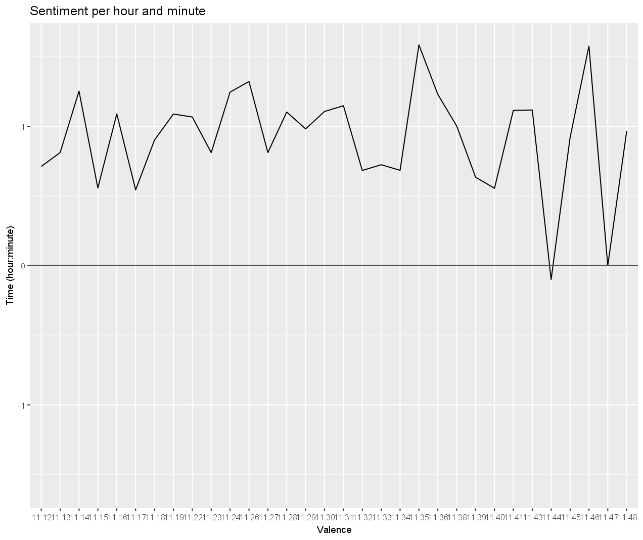
Finally, we can plot the sentiment by time.
ggplot(scores, aes(y = sentiment, x = hourminute, group = 1)) +
  geom_line() +
  geom_hline(yintercept = 0, col = "red") +
  ylim(c(-lim,lim)) +
  labs( x = "Valence", y = "Time (hour:minute)", title = "Sentiment per hour and minute")
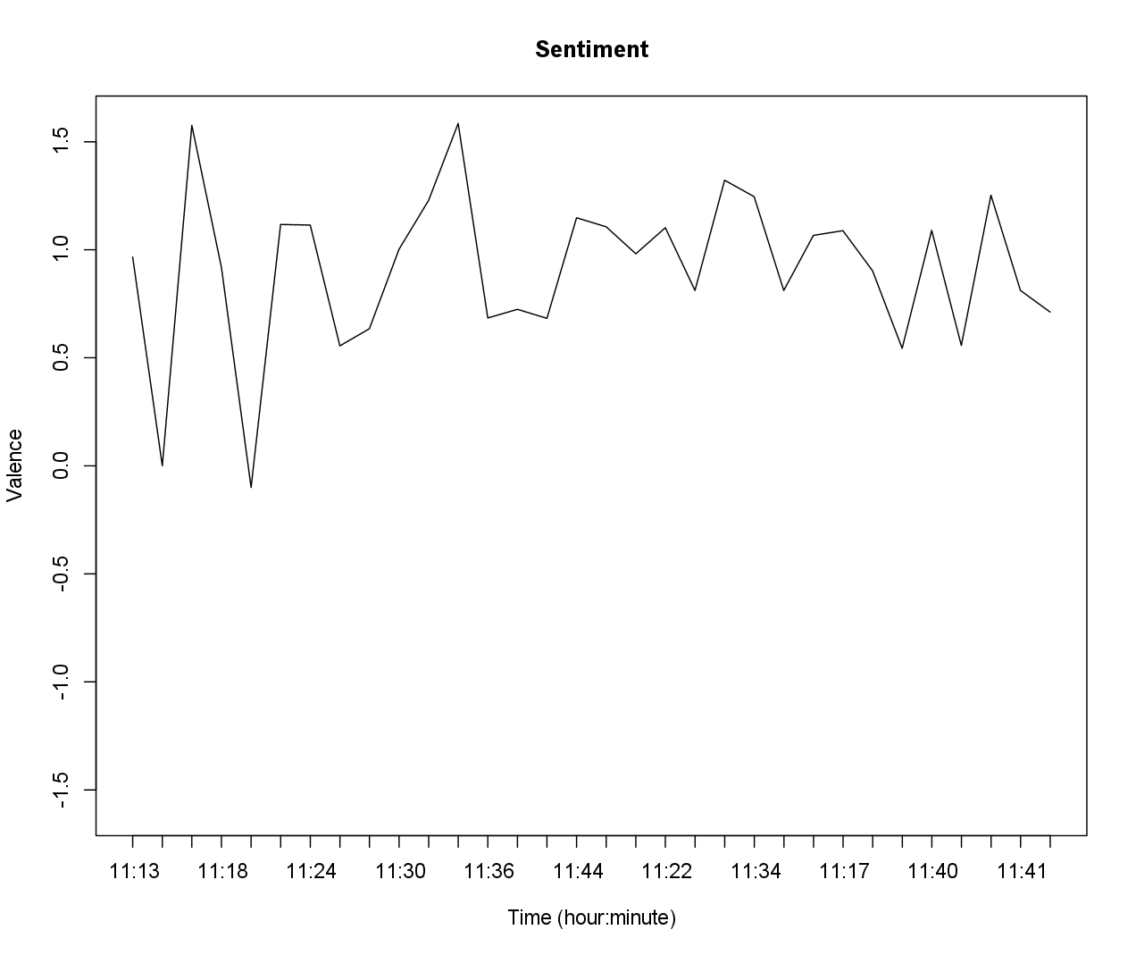
Or in base R:
plot(1:length(scores$sentiment),
     rev(scores$sentiment),
     xaxt="n",
     type="l",
     ylab="Valence",
     xlab="Time (hour:minute)",
     main="Sentiment",
     ylim=c(-lim,lim))
axis(1,at=1:nrow(scores), labels=rev(unique(substr(time,12,16))))
Exercise
Compute the mean score per hour and per minute of the instagramtweets
and store your result as instagram_scores. You do not have to set the encoding or remove special characters of the tweets in this exercise.
Hint: You may need your answer from question 1.1 to extract the text and the datetime of creation from the tweets.
To download the instagramtweets dataset click
here2.
Assume that:
- The
instagramtweetsare given. - The
dictionaryis given. - The lubridate package is loaded.