p_load(AUC, caret)
Labels
We transform the labels to 0 and 1. Note that the dependent variable is -1 and +1, compared to 0 and 1 otherwise. In general, it does not matter whether you use one or the other since the performance will stay the same. However, in computer science -1 and +1 are preferred and in statistics 0 and 1.
y_train <- as.factor(ifelse(train$label==-1, 0,1))
y_test <- as.factor(ifelse(test$label==-1, 0,1))
Logistic regression
We will apply logistic regression.
LR <- glm(y_train ~., data = as.data.frame(trainer$v),family = "binomial")
LR
Call:  glm(formula = y_train ~ ., family = "binomial", data = as.data.frame(trainer$v))

Coefficients:
(Intercept)           V1           V2           V3           V4           V5           V6           V7           V8           V9
 -1.353e+15    6.847e+15    6.362e+14   -1.074e+16    2.642e+15    1.946e+15    7.665e+15   -3.235e+15   -4.093e+15   -5.874e+15
        V10          V11          V12          V13          V14          V15          V16          V17          V18          V19
 -2.202e+15    2.476e+15   -7.263e+14    5.029e+15    3.680e+15   -1.781e+15   -3.525e+15   -2.638e+15    3.892e+15   -1.205e+15
        V20
 -1.156e+15

Degrees of Freedom: 56 Total (i.e. Null);  36 Residual
Null Deviance:	    78.58
Residual Deviance: 1081 	AIC: 1123

preds <- predict(LR,tester,type = "response")
AUC
Next, we can calculate the AUC and plot the ROC curve with the AUC package.
AUC::auc(roc(preds,y_test))
[1] 0.6577381
ROC curve
plot(roc(preds,y_test))
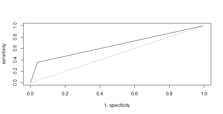
Performance can be better, but if you use more advanced methods (e.g., random forest) or perform regularization (e.g., LASSO), you will already improve the performance. Normally you should use cross-validation to see whether your results are robust. If performance is satisfactory, so you can use this model to extrapolate to unseen results. Sometimes other performance measures are also reported (accuracy). To do so, let’s just use a 0.5 cut-off. Since logistic regression uses the sigmoid function, probabilities are well-calibrated.
preds_lab <- ifelse(preds > 0.5,1,0)
Confusion matrix
xtab <- table(preds_lab, y_test)
confusionMatrix(xtab)
Confusion Matrix and Statistics

         y_test
preds_lab  0  1
        0 23  9
        1  1  5

               Accuracy : 0.7368
                 95% CI : (0.569, 0.866)
    No Information Rate : 0.6316
    P-Value [Acc > NIR] : 0.11814

                  Kappa : 0.3581

 Mcnemar's Test P-Value : 0.02686

            Sensitivity : 0.9583
            Specificity : 0.3571
         Pos Pred Value : 0.7188
         Neg Pred Value : 0.8333
             Prevalence : 0.6316
         Detection Rate : 0.6053
   Detection Prevalence : 0.8421
      Balanced Accuracy : 0.6577

       'Positive' Class : 0
From the confusion matrix, we can conclude that the results are good in terms of accuracy. However, we see that we are better in detecting positive comments (sensitivity) than in detecting negative comments (specificity).
Exercise
Apply logistic regression to the oxfam data, compute the AUC value and save
it as auc_oxfam.
To download the SentimentReal dataset click
here1.
To download the oxfam dataset click
here2.
Assume that:
- The variables
train_oxfam,test_oxfam,trainer, andtrainer, that were calculated in the previous exercise, are given.