Vader

In the following exercise we will perform sentiment analysis, using the vader package. Let’s have a look what using this package does on our example from the previous exercise. As always, we start by loading the required packages.

p_load(vader)

Example: mytext

If you have only one document you need to use the get_vader function, while the vader_df function is used for multiple documents. Since our example contains three documents, we use the latter function.

mytext %>% vader_df()
                                                    text                            word_scores compound   pos   neu   neg but_count
1 Do you like analytics?  But I really hate programming.   {0, 0, 0.75, 0, 0, 0, 0, -4.4895, 0}   -0.695 0.123 0.492 0.386         1
2                              Google is my best friend.                    {0, 0, 0, 3.2, 2.2}    0.813 0.712 0.288 0.000         0
3     Do you really like data analytics?  I'm a huge fan {0, 0, 0, 1.793, 0, 0, 0, 0, 1.3, 1.3}    0.750 0.514 0.486 0.000         0

As you can see, the vader package gives more or less the same results as the sentimentr package. However, the total scores are different because another lexicon is used. The compound score is computed by summing the valence scores of each word in the lexicon, adjusted according to the rules, and then normalized to be between -1 (most extreme negative) and +1 (most extreme positive). This is the most useful metric if you want a single unidimensional measure of sentiment for a given sentence. Calling it a ‘normalized, weighted composite score’ is accurate. It is also useful for researchers who would like to set standardized thresholds for classifying sentences as either positive, neutral, or negative. Typical threshold values used in the literature are:

positive sentiment: compound score >= 0.05,
neutral sentiment: (compound score > -0.05) and (compound score < 0.05),
negative sentiment: compound score <= -0.05.

Let’s have a look at the more difficult text.

mytext2 <- c(
  'Do you like analytics?  But I really hate programming :(.',
  'Google is my beeeeeeeest friend!',
  'Do you really like data analytics?  I\'m a huge fan.'
)
mytext2 %>% vader_df()
                                                       text                             word_scores compound   pos   neu  neg but_count
1 Do you like analytics?  But I really hate programming :(. {0, 0, 0.75, 0, 0, 0, 0, -4.4895, 0, 0}   -0.695 0.115 0.525 0.36         1
2                          Google is my beeeeeeeest friend!                       {0, 0, 0, 0, 2.2}    0.541 0.466 0.534 0.00         0
3       Do you really like data analytics?  I'm a huge fan.  {0, 0, 0, 1.793, 0, 0, 0, 0, 1.3, 1.3}    0.750 0.514 0.486 0.00         0

Notice that it did recognize the exclamation mark and the beeeeest, but it downgraded it.

mytext2 <- c(
  'Do you like analytics?  But I really hate programming :(.',
  'Google is my best friend',
  'Do you really like data analytics?  I\'m a huge fan.'
)
mytext2 %>% vader_df()
                                                      text                             word_scores compound   pos   neu  neg  but_count
1 Do you like analytics?  But I really hate programming :(. {0, 0, 0.75, 0, 0, 0, 0, -4.4895, 0, 0}   -0.695 0.115 0.525 0.36         1
2                                  Google is my best friend                     {0, 0, 0, 3.2, 2.2}    0.813 0.712 0.288 0.00         0
3       Do you really like data analytics?  I'm a huge fan.  {0, 0, 0, 1.793, 0, 0, 0, 0, 1.3, 1.3}    0.750 0.514 0.486 0.00         0

Full sentiment analysis

Let’s perform a full sentiment analysis example on Twitter data. We scrape 100 english tweets about Ariana Grande.

token <- get_token()
search.string <- "ArianaGrande"
no.of.tweets <- 100
ArianaGrande_tweets <- get_timeline(search.string, n=no.of.tweets,lang="en", token  = token)
text <- tweets_data(tweets) %>% pull(text)
text <- iconv(text, from = "latin1", to = "ascii", sub = "byte")

First, we will use the textclean package to detect emojis and emoticons. Notice that not all emojis will be detected, so we will later have to delete the remaining ones.

text_clean <- text %>% 
  replace_emoji() %>% 
  replace_emoticon() %>% 
  replace_contraction() %>%
  replace_internet_slang() %>% 
  replace_kern() %>% 
  replace_word_elongation()

Next, we clean the rest of the posts.

cleanText <- function(text) {
  clean_texts <- text %>%
    str_replace_all("<.*>", "") %>%                         # remove remainig emojis
    str_replace_all("&amp;", "") %>%                        # remove &
    str_replace_all("(RT|via)((?:\\b\\W*@\\w+)+)", "") %>%  # remove retweet entities
    str_replace_all("@\\w+", "") %>%                        # remove @ people, replace_tag() also works
    str_replace_all('#', "") %>%                            #remove only hashtag, replace_hash also works
    str_replace_all("[[:punct:]]", "") %>%                  # remove punctuation
    str_replace_all("[[:digit:]]", "") %>%                  # remove digits
    str_replace_all("http\\w+", "") %>%                     # remove html links replace_html() also works
    str_replace_all("[ \t]{2,}", " ") %>%                   # remove unnecessary spaces
    str_replace_all("^\\s+|\\s+$", "") %>%                  # remove unnecessary spaces
    str_trim() %>% 
    str_to_lower()
  return(clean_texts)
}
text_clean <- cleanText(text_clean)

Lemmatization

In a final preprocessing step, we apply lemmatization by using the textstem package. To do so, we create a dictionary from the text. Note that you can use built-in dictionaries for large corpora.

lemma_dictionary_hs <- make_lemma_dictionary(text_clean, engine = 'hunspell')
text_final <- lemmatize_strings(text_clean, dictionary = lemma_dictionary_hs)

Highlighting the sentiment

Finally, we can extract the sentiment of the tweets. By using the highlight function, the output is shown in a clear html output, as is shown in the screenshot below.

sentiment <- text_final %>% get_sentences() %>% sentiment_by()
sentiment %>% highlight()

html

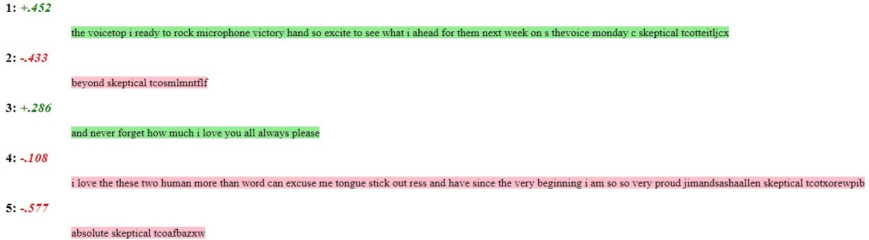
What is strange about the output above?

Exercise

Let's perform another full sentiment analysis on 20 english tweets about Barack Obama. Perform all steps that were performed in the example above. Save the cleaned text, the dictionary, and the final text that will be analysed as text_clean, lemma_dictionary, and text_final, respectively. Also perform a sentiment analysis by using the sentimentR package and the vader package. Store both scores as sentiment_sentimentR and sentiment_vader, respectively.

Hint: You don’t need to use the tweets_data function. You can simply do pull(tweets_BarackObama, text).

token <- get_token()
search.string <- "BarackObama"
no.of.tweets <- 20
tweets_BarackObama <- get_timeline(search.string, n = no.of.tweets, lang = "en", token = token)
save(tweets_BarackObama, file = "tweets_BarackObama.RData")

To download the tweets_BarackObama dataset click here¹.

Assume that:

The Twitter data is given and stored as tweets_BarackObama.
The cleanText function is given.
All the required packages are loaded.