Here we fit a regression tree to the Boston data set. First, we create a training set, and fit the tree to the training data.

library(MASS)
set.seed(8)
train <- sample(1:nrow(Boston), nrow(Boston) / 2)
tree.boston <- tree(medv ~ ., Boston, subset = train)
summary(tree.boston)

Regression tree:
tree(formula = medv ~ ., data = Boston, subset = train)
Variables actually used in tree construction:
[1] "rm"    "lstat" "dis"  
Number of terminal nodes:  8 
Residual mean deviance:  15.16 = 3713 / 245 
Distribution of residuals:
    Min.  1st Qu.   Median     Mean  3rd Qu.     Max. 
-18.3800  -2.3390  -0.1132   0.0000   2.2770  14.3600  

Notice that the output of summary() indicates that only three of the variables have been used in constructing the tree. In the context of a regression tree, the deviance is simply the sum of squared errors for the tree. We now plot the tree.

plot(tree.boston)
text(tree.boston, pretty = 0)

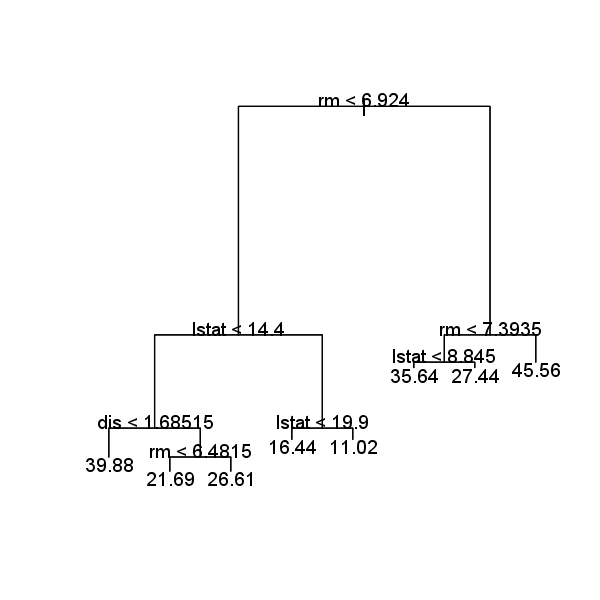
The variable lstat measures the percentage of individuals with lower socioeconomic status. The tree indicates that lower values of lstat correspond to more expensive houses. The tree predicts a median house price of $35,640 for larger homes in suburbs in which residents have high socioeconomic status (rm>=6.924, rm<7.3935 and lstat<8.845).

Questions

• Create a 50-50 train-test split of the Hitters data set. Use a seed value of 1. Store the numeric vector with training data indices in train.idx.
• Fit a regression tree on the training data with Salary as dependent variable and all other variables as independent variables. Store the result in the variable tree.hitters.

MC1: Create a plot of the tree and select the correct answer

• A) a lower value for RBI results in a higher expected value for Salary
• B) a higher value for Errors leads to a higher expected value for Salary
  • 1) Both statements are true.
  • 2) Both statements are false.
  • 3) A is true and B is false.
  • 4) A is false and B is true.

Assume that:

• The ISLR2 and tree libraries have been loaded
• The Hitters dataset has been loaded and attached