We use the e1071 library in R to demonstrate the support vector classifier and the SVM. Another option is the LiblineaR library, which is useful for very large linear problems.

The e1071 library contains implementations for a number of statistical learning methods. In particular, the svm() function can be used to fit a support vector classifier when the argument kernel="linear" is used.

WARNING: The cost argument in the svm() function is the inverse of the hyperparameter $C$ (budget) in the optimization problem discussed in the theory lecture: \(C = \textrm{budget} = \frac{1}{\texttt{cost}}.\) As such, cost refers to the cost of a violation to the margin. When the cost argument is small, then the margins will be wide and many support vectors will be on the margin or will violate the margin. When the cost argument is large, then the margins will be narrow and there will be few support vectors on the margin or violating the margin.

We now use the svm() function to fit the support vector classifier for a given value of the cost parameter. Here we demonstrate the use of this function on a two-dimensional example so that we can plot the resulting decision boundary. We begin by generating the observations, which belong to two classes.

set.seed(1)
x <- matrix(rnorm(20 * 2), ncol = 2)
y <- c(rep(-1, 10), rep(1, 10))
x[y == 1,] <- x[y == 1,] + 1

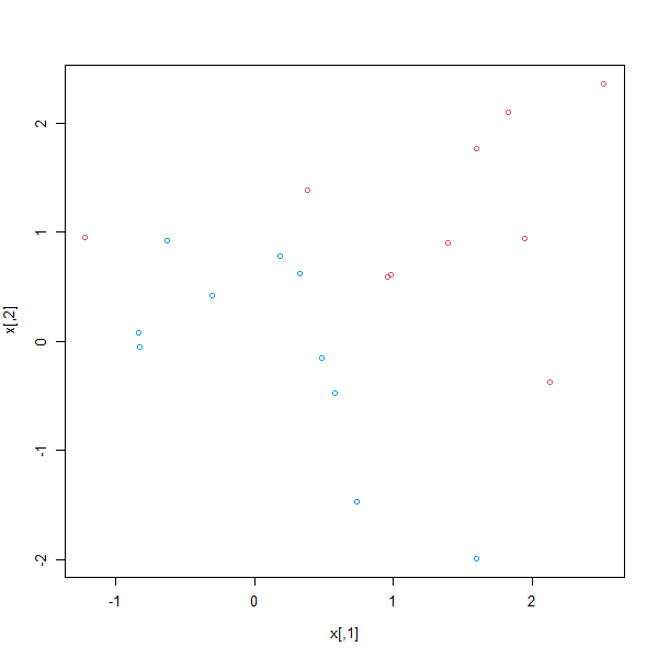
We begin by checking whether the classes are linearly separable.

plot(x, col = (3 - y))

They are not. Next, we fit the support vector classifier. Note that in order for the svm() function to perform classification (as opposed to SVM-based regression), we must encode the response as a factor variable. We now create a data frame with the response coded as a factor.

dat <- data.frame(x = x, y = as.factor(y))
library(e1071)
svmfit <- svm(y ~ ., data = dat, kernel = "linear", cost = 10, scale = FALSE)

The argument scale=FALSE tells the svm() function not to scale each feature to have mean zero or standard deviation one; depending on the application, one might prefer to use scale=TRUE.

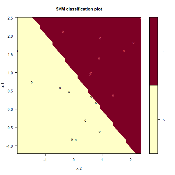
We can now plot the support vector classifier obtained:

plot(svmfit, dat)

Note that the two arguments to the plot.svm() function are the output of the call to svm(), as well as the data used in the call to svm(). The region of feature space that will be assigned to the −1 class is shown in yellow, and the region that will be assigned to the +1 class is shown in red. The decision boundary between the two classes is linear (because we used the argument kernel="linear"), though due to the way in which the plotting function is implemented in this library the decision boundary looks somewhat jagged in the plot. We see that in this case only one observation is misclassified. (Note that here the second feature is plotted on the x-axis and the first feature is plotted on the y-axis, in contrast to the behavior of the usual plot() function in R.) The support vectors are plotted as crosses and the remaining observations are plotted as circles; we see here that there are seven support vectors. We can determine their identities as follows:

svmfit$index

[1]  1  2  5  7 14 16 17

We can obtain some basic information about the support vector classifier fit using the summary() command:

summary(svmfit)

Call:
svm(formula = y ~ ., data = dat, 
    kernel = "linear", cost = 10, 
    scale = FALSE)
Parameters:
   SVM-Type:  C-classification 
 SVM-Kernel:  linear 
       cost:  10 
Number of Support Vectors:  7
 ( 4 3 )
Number of Classes:  2 
Levels: 
 -1 1

This tells us, for instance, that a linear kernel was used with cost=10, and that there were seven support vectors, four in one class and three in the other.

What if we instead used a smaller value of the cost parameter?

Questions

• Create a SVM with a linear kernel, no scaling and the cost parameter equal to 0.1. Store the model in svmfit.
• Look at the summary of the model, how many support vectors are there? Store the total number of support vectors in nSV.

You can find the total number of support vectors within the tot.nSV attribute of svmfit

MC1: If we were to choose a smaller value of the cost parameter, what would happen?
1) The margin becomes wider, so we will obtain a larger number of support vectors
2) The margin becomes wider, so we will obtain a smaller number of support vectors
3) The margin becomes thinner, so we will obtain a larger number of support vectors
4) The margin becomes thinner, so we will obtain a smaller number of support vectors
5) The cost parameter has no influence on the width of the margin nor the number of support vectors

---

Assume that:

• The e1071 library has been loaded