Inferentie

Er zijn meerdere interactie termen in het model. We kunnen deze eerst samen testen a.d.h.v. van de resultaten uit de anova tabel.

library(car)
Anova(rats3, type="III")

## Anova Table (Type III tests)
## 
## Response: 1/time
##                Sum Sq Df  F value    Pr(>F)    
## (Intercept)  0.247383  1 103.0395 4.158e-12 ***
## poison       0.111035  2  23.1241 3.477e-07 ***
## treat        0.035723  3   4.9598  0.005535 ** 
## poison:treat 0.015708  6   1.0904  0.386733    
## Residuals    0.086431 36                       
## ---
## Signif. codes:  0 '***' 0.001 '**' 0.01 '*' 0.05 '.' 0.1 ' ' 1

Verwijderen van niet-significante interactie.

De interactie tussen gif en behandeling is niet significant op het 5% niveau.

Een veelgebruikte methode is om de niet-significante interactie te verwijderen uit het model.

We verkrijgen dan een additief model wat toelaat om de effecten van de twee factoren afzonderlijk te bestuderen.

rats4 <- lm(1/time~poison + treat, rats)
plot(rats4)

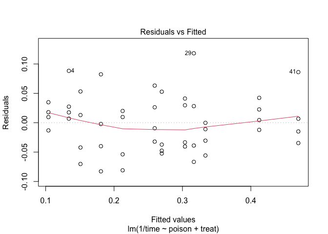
We zien wel iets meer afwijkingen in de residu plot.

Anova(rats4, type="III")

## Anova Table (Type III tests)
## 
## Response: 1/time
##              Sum Sq Df F value    Pr(>F)    
## (Intercept) 0.58219  1 239.399 < 2.2e-16 ***
## poison      0.34877  2  71.708 2.865e-14 ***
## treat       0.20414  3  27.982 4.192e-10 ***
## Residuals   0.10214 42                      
## ---
## Signif. codes:  0 '***' 0.001 '**' 0.01 '*' 0.05 '.' 0.1 ' ' 1

De anova tabel toont dat het effect van gif en behandeling beiden extreem siginficant zijn (beide \(p<< 0.001\)).

Het additieve model laat toe om de effecten van het type gif en de behandeling afzonderlijke te bestuderen via een post-hoc analyse.

library(multcomp)
comparisons <- glht(rats4, linfct = mcp(poison = "Tukey", treat="Tukey"))
summary(comparisons)

## 
##   Simultaneous Tests for General Linear Hypotheses
## 
## Multiple Comparisons of Means: Tukey Contrasts
## 
## 
## Fit: lm(formula = 1/time ~ poison + treat, data = rats)
## 
## Linear Hypotheses:
##                       Estimate Std. Error t value Pr(>|t|)    
## poison: II - I == 0    0.04686    0.01744   2.688  0.07347 .  
## poison: III - I == 0   0.19964    0.01744  11.451  < 0.001 ***
## poison: III - II == 0  0.15278    0.01744   8.763  < 0.001 ***
## treat: B - A == 0     -0.16574    0.02013  -8.233  < 0.001 ***
## treat: C - A == 0     -0.05721    0.02013  -2.842  0.05091 .  
## treat: D - A == 0     -0.13583    0.02013  -6.747  < 0.001 ***
## treat: C - B == 0      0.10853    0.02013   5.391  < 0.001 ***
## treat: D - B == 0      0.02991    0.02013   1.485  0.61547    
## treat: D - C == 0     -0.07862    0.02013  -3.905  0.00276 ** 
## ---
## Signif. codes:  0 '***' 0.001 '**' 0.01 '*' 0.05 '.' 0.1 ' ' 1
## (Adjusted p values reported -- single-step method)

confint(comparisons)

## 
##   Simultaneous Confidence Intervals
## 
## Multiple Comparisons of Means: Tukey Contrasts
## 
## 
## Fit: lm(formula = 1/time ~ poison + treat, data = rats)
## 
## Quantile = 2.8498
## 95% family-wise confidence level
##  
## 
## Linear Hypotheses:
##                       Estimate   lwr        upr       
## poison: II - I == 0    0.0468641 -0.0028223  0.0965506
## poison: III - I == 0   0.1996425  0.1499561  0.2493289
## poison: III - II == 0  0.1527784  0.1030919  0.2024648
## treat: B - A == 0     -0.1657402 -0.2231132 -0.1083673
## treat: C - A == 0     -0.0572135 -0.1145865  0.0001594
## treat: D - A == 0     -0.1358338 -0.1932068 -0.0784609
## treat: C - B == 0      0.1085267  0.0511538  0.1658996
## treat: D - B == 0      0.0299064 -0.0274665  0.0872794
## treat: D - C == 0     -0.0786203 -0.1359932 -0.0212473

plot(comparisons,yaxt="none")
contrastNames <- c("II-I","III-I","III-II","B-A","C-A","D-A","C-B","D-B","D-C")
axis(2,at=c(length(contrastNames):1), labels=contrastNames,las=2)

Niet-significante interactie term in het model weerhouden

Het aanvaarden van de null hypothese dat er geen interactie is, is een zwakke conclusie. Het zou immers kunnen dat de power van het experiment te klein is om de interactie op te pikken. We kunnen er ook voor kiezen om de niet significante interactie term in het model te laten.

Als de interactie significant zou zijn geweest, betekent dit dat het effect van het gif op de snelheid van sterven afhangt van de behandeling en vice versa. Dan kunnen we het effect van het type gif en de behandeling op de overlevingstijd niet afzonderlijk bestuderen.

ExploreModelMatrix::VisualizeDesign(rats,~poison*treat)$plot

## [[1]]

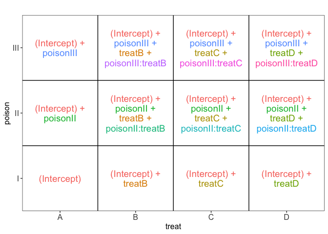
We zouden dan het effect van het type gif afzonderlijk moeten bestuderen voor elke behandeling:

Voor behandeling A moeten we dan volgende nulhypotheses toetsen:

II-I: \(H_0: \beta_{II}=0\)
III-I: \(H_0: \beta_{III}=0\)
III-II: \(H_0: \beta_{III}-\beta_{II}=0\)

Voor behandeling B:

II-I: \(H_0: \beta_{II}+\beta_{II:B}=0\)
III-I: \(H_0: \beta_{III}+\beta_{III:B}=0\)
III-II: \(H_0: \beta_{III}+\beta_{III:B}-\beta_{II}-\beta_{II:B}=0\)

Voor behandeling C:

II-I: \(H_0: \beta_{II}+\beta_{II:C}=0\)
III-I: \(H_0: \beta_{III}+\beta_{III:C}=0\)
III-II: \(H_0: \beta_{III}+\beta_{III:C}-\beta_{II}-\beta_{II:C}=0\)

Voor behandeling D:

II-I: \(H_0: \beta_{II}+\beta_{II:D}=0\)
III-I: \(H_0: \beta_{III}+\beta_{III:D}=0\)
III-II: \(H_0: \beta_{III}+\beta_{III:D}-\beta_{II}-\beta_{II:D}=0\)

Het zelfde geldt wanneer we het effect van de behandeling bestuderen:

Voor gif I toetsen we dan nulhypothese

B-A: \(H_0: \beta_{B}=0\)
C-A: \(H_0: \beta_{C}=0\)
D-A: \(H_0: \beta_{D}=0\)
C-B: \(H_0: \beta_{C}-\beta_{B}=0\)
D-B: \(H_0: \beta_{D}-\beta_{B}=0\)
D-C: \(H_0: \beta_{D}-\beta_{C}=0\)

Gif II

B-A: \(H_0: \beta_{B}+\beta_{II:B}=0\)
C-A: \(H_0: \beta_{C}+\beta_{II:C}=0\)
D-A: \(H_0: \beta_{D}+\beta_{II:D}=0\)
C-B: \(H_0: \beta_{C}+\beta_{II:C}-\beta_{B}-\beta_{II:B}=0\)
D-B: \(H_0: \beta_{D}+\beta_{II:D}-\beta_{B}-\beta_{II:B}=0\)
D-C: \(H_0: \beta_{D}+\beta_{II:D}-\beta_{C}-\beta_{II:C}=0\)

Gif III

B-A: \(H_0: \beta_{B}+\beta_{III:B}=0\)
C-A: \(H_0: \beta_{C}+\beta_{III:C}=0\)
D-A: \(H_0: \beta_{D}+\beta_{II:D}=0\)
C-B: \(H_0: \beta_{C}+\beta_{III:C}-\beta_{B}-\beta_{III:B}=0\)
D-B: \(H_0: \beta_{D}+\beta_{III:D}-\beta_{B}-\beta_{III:B}=0\)
D-C: \(H_0: \beta_{D}+\beta_{III:D}-\beta_{C}-\beta_{III:C}=0\)

comparisonsInt <- glht(rats3, linfct = c(
  "poisonII = 0",
  "poisonIII = 0",
  "poisonIII - poisonII = 0",
  "poisonII + poisonII:treatB = 0",
  "poisonIII + poisonIII:treatB = 0",
  "poisonIII + poisonIII:treatB - poisonII- poisonII:treatB = 0",  
  "poisonII + poisonII:treatC = 0",
  "poisonIII + poisonIII:treatC = 0",
  "poisonIII + poisonIII:treatC - poisonII- poisonII:treatC = 0",  
  "poisonII + poisonII:treatD = 0",
  "poisonIII + poisonIII:treatD = 0",
  "poisonIII + poisonIII:treatD - poisonII- poisonII:treatD = 0",  
  "treatB = 0",
  "treatC = 0",
  "treatD = 0",
  "treatC - treatB = 0",
  "treatD - treatB = 0",
  "treatD - treatC = 0",
  "treatB + poisonII:treatB = 0",
  "treatC + poisonII:treatC = 0",
  "treatD + poisonII:treatD = 0",
  "treatC + poisonII:treatC - treatB - poisonII:treatB = 0",
  "treatD + poisonII:treatD - treatB - poisonII:treatB = 0",
  "treatD + poisonII:treatD - treatC - poisonII:treatC = 0",
  "treatB + poisonIII:treatB = 0",
  "treatC + poisonIII:treatC = 0",
  "treatD + poisonIII:treatD = 0",
  "treatC + poisonIII:treatC - treatB - poisonIII:treatB = 0",
  "treatD + poisonIII:treatD - treatB - poisonIII:treatB = 0",
  "treatD + poisonIII:treatD - treatC - poisonIII:treatC = 0")
)

contrastNames<-
  c(paste(rep(LETTERS[1:4],each=3),rep(apply(combn(c("I","II","III"),2)[2:1,],2,paste,collapse="-") ,4),sep=": "),
    paste(rep(c("I","II","III"),each=6),rep(apply(combn(c(LETTERS[1:4]),2)[2:1,],2,paste,collapse="-") ,3),sep=": "))

plot(comparisonsInt,yaxt="none")
axis(2,at=c(length(contrastNames):1), labels=contrastNames,las=2)

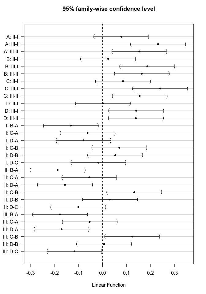
In onze studie was de interactie echter niet significant. Het effect van het gif (II-I, III-I en III- II) verandert dus niet significant volgens de behandeling (A, B, C, en D) en vice versa. Voor onze dataset lijkt het dus zinvol om

de effectgrootte voor de pairsgewijze vergelijkingen tussen de verschillende giffen (II-I, III-I en III- II) te schatten door ze uit te middelen over alle behandelingen (A, B, C, en D), en,
de effectgrootte voor de pairsgewijze vergelijkingen tussen de verschillende behandelingen (B-A, C-A, D-A, C-B, D-B en D-C) te schatten door ze uit te middelen over alle giffen (I, II, III).

Dat zou ons gelijkaardige schattingen van de effectgroottes moeten geven als deze voor het additieve model waarbij we de interactie term uit het model hadden geweerd.

B.v. voor gif III vs gif II zou dat in volgende contrast resulteren:

III-II:

\[H_0: \begin{array}{l} \frac{\beta_{III}-\beta_{II}}{4} + \\ \quad \frac{\beta_{III} + \beta_{III:B}-\beta_{II} - \beta_{II:B}}{4} + \\ \quad \quad \frac{\beta_{III} + \beta_{III:C}-\beta_{II} - \beta_{II:C}}{4} + \\ \quad \quad \quad \frac{\beta_{III} + \beta_{III:D}-\beta_{II} - \beta_{II:D}}{4}=0 \end{array}\] \[H_0:\beta_{III} + \frac{1}{4} \times \beta_{III:B} + \frac{1}{4} \times\beta_{III:C} + \frac{1}{4} \times\beta_{III:D} -\beta_{II} - \frac{1}{4} \times\beta_{II:B} - \frac{1}{4} \times\beta_{II:C} - \frac{1}{4} \times\beta_{II:D}=0\]

We schatten met onderstaande code alle gemiddelde contrasten a.d.h.v. het model met interactie.

contrasts <- c(
  "poisonII + 1/4*poisonII:treatB + 1/4*poisonII:treatC + 1/4*poisonII:treatD = 0",
  "poisonIII + 1/4*poisonIII:treatB + 1/4*poisonIII:treatC + 1/4*poisonIII:treatD= 0",
  "poisonIII + 1/4*poisonIII:treatB + 1/4*poisonIII:treatC + 1/4*poisonIII:treatD - poisonII - 1/4*poisonII:treatB - 1/4*poisonII:treatC - 1/4*poisonII:treatD = 0",
  "treatB + 1/3*poisonII:treatB + 1/3*poisonIII:treatB = 0",
  "treatC + 1/3*poisonII:treatC + 1/3*poisonIII:treatC = 0",
  "treatD + 1/3*poisonII:treatD + 1/3*poisonIII:treatD = 0",
  "treatC + 1/3*poisonII:treatC + 1/3*poisonIII:treatC - treatB - 1/3*poisonII:treatB - 1/3*poisonIII:treatB = 0",
  "treatD + 1/3*poisonII:treatD + 1/3*poisonIII:treatD  - treatB - 1/3*poisonII:treatB - 1/3*poisonIII:treatB = 0",
  "treatD + 1/3*poisonII:treatD + 1/3*poisonIII:treatD  - treatC - 1/3*poisonII:treatC - 1/3*poisonIII:treatC = 0") 


comparisonsInt2 <- glht(rats3, linfct = contrasts
)
plot(comparisonsInt2,yaxt="none")
contrastNames <- c("II-I","III-I","III-II","B-A","C-A","D-A","C-B","D-B","D-C")
axis(2,at=c(length(contrastNames):1), labels=contrastNames,las=2)

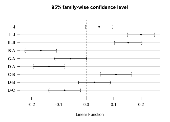
De geschatte effectgroottes zijn inderdaad exact gelijk als bij het model zonder interactie omdat het experiment gebalanceerd is.

De standaard errors verschillen wel lichtjes. Dat is het gevolg van de errors die verschillen tussen beiden modellen alsook het aantal vrijheidsgraden van de errors (n-p).

data.frame(Additive_coef=summary(comparisons)$test$coef,Additive_se=summary(comparisons)$test$sigma,Int_coef=summary(comparisonsInt2)$test$coef,int_se=summary(comparisonsInt2)$test$sigma) %>% round(3)

##                  Additive_coef Additive_se Int_coef int_se
## poison: II - I           0.047       0.017    0.047  0.017
## poison: III - I          0.200       0.017    0.200  0.017
## poison: III - II         0.153       0.017    0.153  0.017
## treat: B - A            -0.166       0.020   -0.166  0.020
## treat: C - A            -0.057       0.020   -0.057  0.020
## treat: D - A            -0.136       0.020   -0.136  0.020
## treat: C - B             0.109       0.020    0.109  0.020
## treat: D - B             0.030       0.020    0.030  0.020
## treat: D - C            -0.079       0.020   -0.079  0.020