Topics and Terms

After creating the LDA model, we can inspect the topics and terms. We’ll use the tidy function to neatly output the beta matrix.

(topic_term <- tidy(topicmodel, matrix = 'beta'))

# A tibble: 9,184 x 3
   topic    term            beta
   <int>    <chr>           <dbl>
 1     1    pay        1.52e- 50
 2     2    pay        4.70e- 57
 3     3    pay        1.22e-  2
 4     4    pay        5.55e-177
 5     1    black      3.25e- 28
 6     2    black      5.65e-  4
 7     3    black      1.32e-156
 8     4    black      2.61e-  3
 9     1    history    1.12e-  3
10     2    history    1.47e-  3
# ... with 9,174 more rows

Each row represents a topic per term. For example, pay has a probability of 1.52e-50 to belong to topic 1.

Identifying Top Terms per Topic

We can also identify the top ten terms per topic.

top_terms <- topic_term %>%
  group_by(topic) %>%
  top_n(10, beta) %>%
  ungroup() %>%
  arrange(topic, desc(beta))
top_terms

# A tibble: 40 x 3
   topic    term              beta
   <int>    <chr>             <dbl>
 1     1    republicans     0.0229
 2     1    roe             0.0206
 3     1    house           0.0152
 4     1    social          0.0148
 5     1    security        0.0140
 6     1    democrats       0.0133
 7     1    wade            0.0129
 8     1    codify          0.0124
 9     1    law             0.0121
10     1    protect         0.0119
# ... with 30 more rows

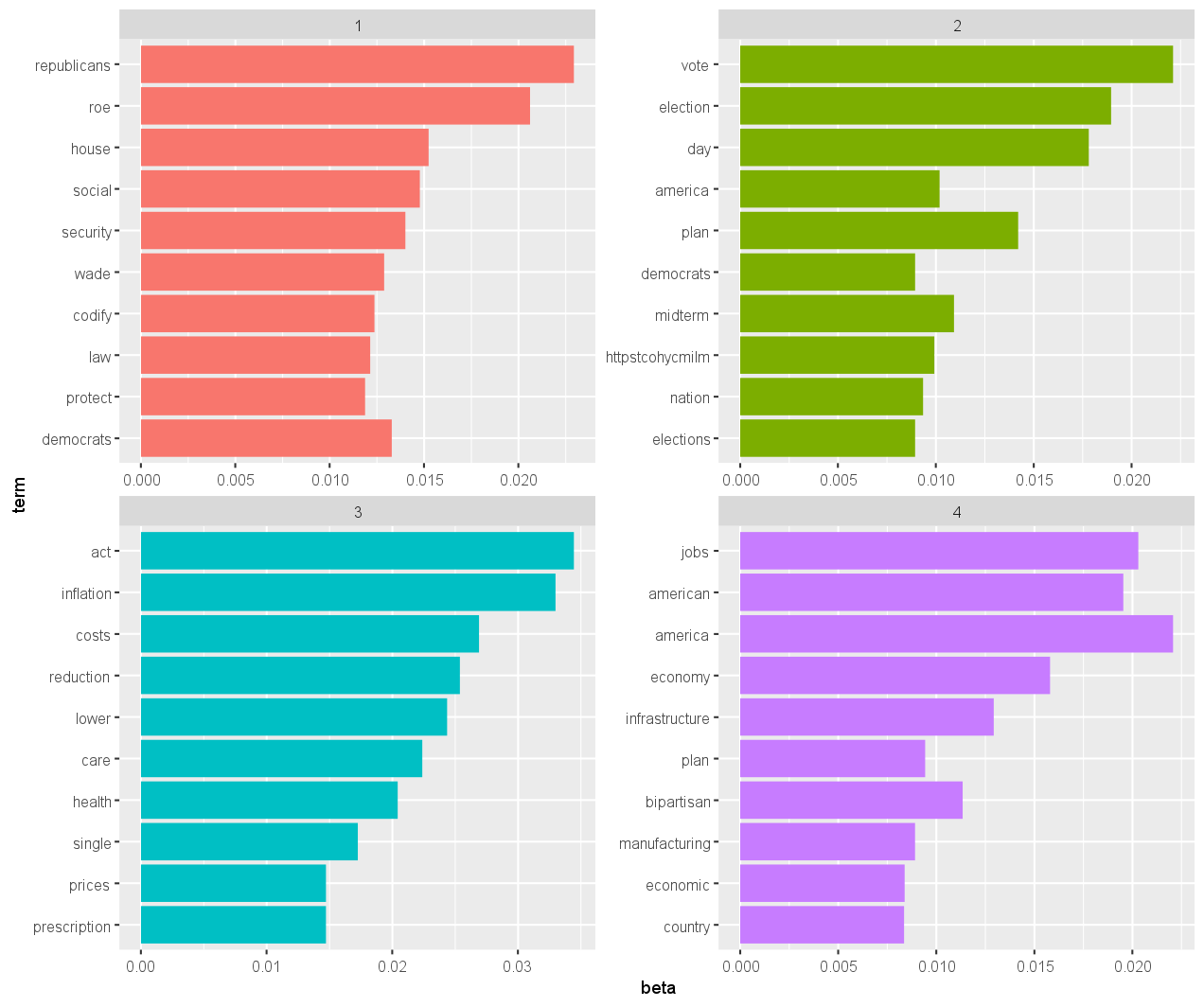
Visualizing Top Terms

These top ten terms per topic can be visualized using a bar plot.

top_terms %>%
  mutate(term = reorder(term, beta)) %>%
  ggplot(aes(term, beta, fill = factor(topic))) +
  geom_col(show.legend = FALSE) +
  facet_wrap(~ topic, scales = "free") +
  coord_flip()

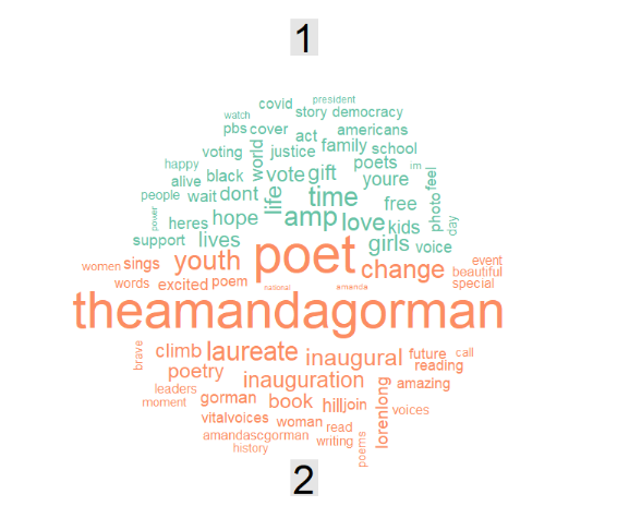
Creating a Word Cloud

We can also create a word cloud for a more intuitive understanding of the top terms.

topic_term %>% 
  group_by(topic) %>% 
  top_n(50, beta) %>% 
  pivot_wider(term, topic, values_from = "beta", names_prefix = 'topic', values_fill = 0) %>% 
  column_to_rownames("term") %>%  
  comparison.cloud(colors = brewer.pal(3, "Set2")) 

To download the topicmodel click: here¹

Assume that:

• The topicmodel from the previous exercise has been loaded.
• All the packages to perform topic modeling have been loaded.