Now we will perform LDA on the Smarket data. In R, we fit a LDA model
using the lda() function, which is part of the MASS library.
Notice that the syntax for the lda() function is identical to that of lm(),
and to that of
glm() except for the absence of the family option. We fit the model using
only the observations before 2005.
> library(MASS)
> library(ISLR2)
> attach(Smarket)
> train <- (Year < 2005)
> lda.fit <- lda(Direction ~ Lag1 + Lag2, data = Smarket, subset = train)
> lda.fit
Call:
lda(Direction ~ Lag1 + Lag2, data = Smarket, subset = train)
Prior probabilities of groups:
Down Up
0.491984 0.508016
Group means:
Lag1 Lag2
Down 0.04279022 0.03389409
Up -0.03954635 -0.03132544
Coefficients of linear discriminants:
LD1
Lag1 -0.6420190
Lag2 -0.5135293
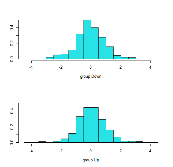
> plot(lda.fit)
The LDA output indicates that \(\hat\pi_1 = 0.492\) and \(\hat\pi_2 = 0.508\) ; in other words,
49.2% of the training observations correspond to days during which the
market went down. It also provides the group means; these are the average
of each predictor within each class, and are used by LDA as estimates
of \(\mu_k\). These suggest that there is a tendency for the previous 2 days’
returns to be negative on days when the market increases, and a tendency
for the previous days’ returns to be positive on days when the market
declines. The coefficients of linear discriminants output provides the linear
combination of Lag1 and Lag2 that are used to form the LDA decision rule.
In other words, these are the multipliers of the elements of \(X = x\) in
(4.19). If -0.642×Lag1-0.514×Lag2 is large, then the LDA classifier will
predict a market increase, and if it is small, then the LDA classifier will
predict a market decline. The plot() function produces plots of the linear
discriminants, obtained by computing −0.642 × Lag1 − 0.514 × Lag2 for
each of the training observations.
Try modifying the current lda model by adding the Lag3 variable:
Assume that:
- The
ISLR2andMASSlibraries have been loaded - The
Smarketdataset has been loaded and attached