Next, we use the boot() function to compute the standard errors of 1,000
bootstrap estimates for the intercept and slope terms.
> boot(Auto, boot.fn, 1000)

ORDINARY NONPARAMETRIC BOOTSTRAP

Call:
boot(data = Auto, statistic = boot.fn, R = 1000)

Bootstrap Statistics :
      original        bias    std. error
t1* 39.9358610  0.0544513229 0.841289790
t2* -0.1578447 -0.0006170901 0.007343073
This indicates that the bootstrap estimate for \(SE(\hat\beta_0)\) is 0.841, and that
the bootstrap estimate for \(SE(\hat\beta_1)\) is 0.00734. As discussed in Section 3.1.2,
standard formulas can be used to compute the standard errors for the
regression coefficients in a linear model. These can be obtained using the
summary() function.
> summary(lm(mpg ~ horsepower, data = Auto))$coef
              Estimate  Std. Error   t value      Pr(>|t|)
(Intercept) 39.9358610 0.717498656  55.65984 1.220362e-187
horsepower  -0.1578447 0.006445501 -24.48914  7.031989e-81
The standard error estimates for \(\hat\beta_0\) and \(\hat\beta_1\) obtained using the formulas:
\[\hat\beta_1 = \frac{\sum_{i=1}^{n}(x_i-\bar x)(y_i-\bar y)}{\sum_{i=1}^{n}(x_i-\bar x)^2}, \hat\beta_0 = \hat y - \hat \beta_1 \bar x\]are 0.717 for the intercept and 0.00645 for the slope. Interestingly, these are somewhat different from the estimates obtained using the bootstrap. Does this indicate a problem with the bootstrap? In fact, it suggests the opposite. Recall that the standard formulas:
\[SE(\hat\beta_0)^2 = \sigma^2[\frac{1}{n}+\frac{\bar x^2}{\sum_{i = 1}^{n}(x_i-\bar x^2)}] , SE(\hat\beta_1)^2 = \frac{\sigma^2}{\sum_{i = 1}^{n}(x_i-\bar x^2)}\]rely on certain assumptions. For example, they depend on the unknown parameter \(\sigma^2\), the noise variance. We then estimate \(\sigma^2\) using the RSS. Now although the formula for the standard errors do not rely on the linear model being correct, the estimate for \(\sigma^2\) does.

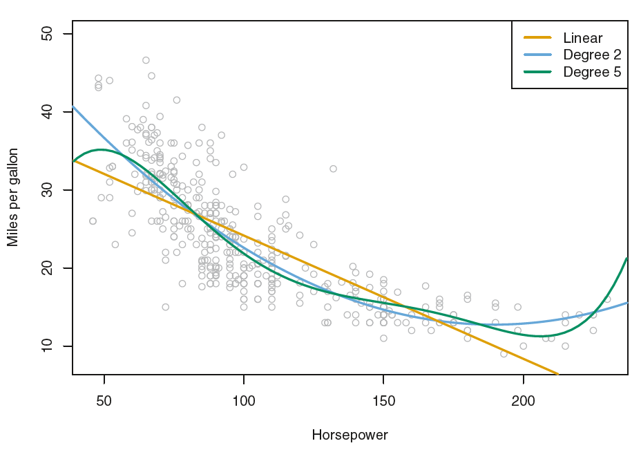
Here we see that there is a non-linear relationship in the data, and
so the residuals from a linear fit (yellow line) will be inflated, and so will \(\hat\sigma^2\). Secondly,
the standard formulas assume (somewhat unrealistically) that the \(x_i\) are
fixed, and all the variability comes from the variation in the errors \(\epsilon_i\). The
bootstrap approach does not rely on any of these assumptions, and so it is
likely giving a more accurate estimate of the standard errors of \(\hat\beta_0\) and \(\hat\beta_1\)
than is the summary() function.
Below we compute the bootstrap standard error estimates and the standard linear regression estimates that result from fitting the quadratic model to the data. Since this model provides a good fit to the data (blue line), there is now a better correspondence between the bootstrap estimates and the standard estimates of \(SE(\hat\beta_0)\), \(SE(\hat\beta_1)\) and \(SE(\hat\beta_2)\).
> boot.fn <- function(data, index)
+ coefficients(lm(mpg ~ horsepower + I(horsepower^2), data = data,
+ subset = index))
> set.seed(1)
>
> boot(Auto, boot.fn, 1000)

ORDINARY NONPARAMETRIC BOOTSTRAP

Call:
boot(data = Auto, statistic = boot.fn, R = 1000)

Bootstrap Statistics :
        original        bias     std. error
t1* 56.900099702  3.511640e-02 2.0300222526
t2* -0.466189630 -7.080834e-04 0.0324241984
t3*  0.001230536  2.840324e-06 0.0001172164
> summary(lm(mpg ~ horsepower + I(horsepower^2), data = Auto))$coef
                    Estimate   Std. Error   t value      Pr(>|t|)
(Intercept)     56.900099702 1.8004268063  31.60367 1.740911e-109
horsepower      -0.466189630 0.0311246171 -14.97816  2.289429e-40
I(horsepower^2)  0.001230536 0.0001220759  10.08009  2.196340e-21
Try to create 10 bootstrap estimates for your own and store them in bootstrap:
Assume that:
- The
ISLR2andbootlibraries have been loaded - The
Autodataset has been loaded and attached