In this problem, you will generate simulated data, and then perform PCA and \(K\)-means clustering on the data.

First we generate a simulated data set with 20 observations in each of three classes (i.e. 60 observations total), and 50 variables.

set.seed(2)
x <- matrix(rnorm(20 * 3 * 50, mean = 0, sd = 0.3), ncol = 50)
x[1:20, 2] <- 1
x[21:40, 1] <- 2
x[21:40, 2] <- 2
x[41:60, 1] <- 1
true.labels <- c(rep(1, 20), rep(2, 20), rep(3, 20))

Questions

1. Perform PCA on the 60 observations and store the model in pr.out. Do not scale the data.

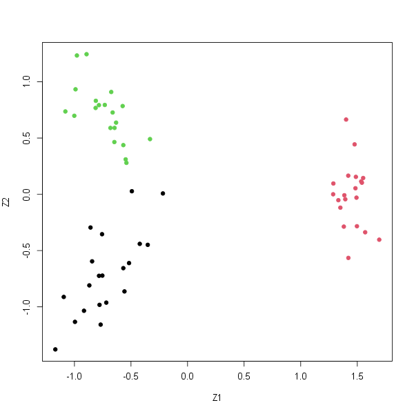
2. Plot the first two principal component score vectors. Use a different color to indicate the observations in each of the three classes.

   The plot should look something like this:

   

3. Perform \(K\)-means clustering of the observations with \(K = 3\) with the nstart argument set to 20. Store the model in km.out3. How well do the clusters that you obtained in \(K\)-means clustering compare to the true class labels?

4. Perform \(K\)-means clustering with \(K = 2\) with the nstart argument set to 20. Store the model in km.out2. How do these results compare to those obtained in 3?

5. Now perform \(K\)-means clustering with \(K = 4\) with the nstart argument set to 20. Store the model in km.out4. How do these results compare to those obtained in 3?

6. Now perform \(K\)-means clustering with \(K = 3\) with the nstart argument set to 20 on the first two principal component score vectors, rather than on the raw data. That is, perform \(K\)-means clustering on the 60x2 matrix of which the first column is the first principal component score vector, and the second column is the second principal component score vector. Store the model in km.out.pca. How do these results compare to those obtained in 3?

7. Using the scale() function, perform \(K\)-means clustering with \(K = 3\) with the nstart argument set to 20 on the data after scaling each variable to have standard deviation one. Store the model in km.out.sd. How do these results compare to those obtained in 3?