The prcomp() function also outputs the standard deviation of each principal component. For instance, on the USArrests data set, we can access these standard deviations as follows:

> pr.out$sdev
[1] 1.5748783 0.9948694 0.5971291 0.4164494

The variance explained by each principal component is obtained by squaring these:

> pr.var <- pr.out$sdev^2
> pr.var
[1] 2.4802416 0.9897652 0.3565632 0.1734301

To compute the proportion of variance explained by each principal component, we simply divide the variance explained by each principal component by the total variance explained by all four principal components:

> pve <- pr.var / sum(pr.var)
> pve
[1] 0.62006039 0.24744129 0.08914080 0.04335752

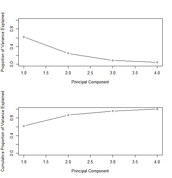
We see that the first principal component explains 62.0% of the variance in the data, the next principal component explains 24.7% of the variance, and so forth. We can plot the PVE explained by each component, as well as the cumulative PVE, as follows:

par(mfrow = c(2, 1))
plot(pve, xlab = "Principal Component", ylab = "Proportion of Variance Explained", ylim = c(0, 1), type = 'b')
plot(cumsum(pve), xlab = "Principal Component", ylab = "Cumulative Proportion of Variance Explained", ylim = c(0, 1), type = 'b')

Note that the function cumsum() computes the cumulative sum of the elements of a numeric vector. For instance:

> a <- c(1, 2, 8, -3)
> cumsum(a)
[1]  1  3 11  8

Question

MC1:
If we would only use the first two principal components, how much of the variance would we be able to explain?

1. 62.0%
2. 24.7%
3. 86.7%
4. 100.0%