STEP 5: Dimensionality reduction

In the fifth step, we will use singular value decomposition as dimensionality reduction technique. Before we can use SVD, we have to transform the data to a matrix. Let’s start from the dtm_reviews_dense variable.

reviews_mat <- as.matrix(dtm_reviews_dense)

dim(reviews_mat)

[1]   5 169

Center the data when the features have very different scalings. We do not want to take scaling into account when considering the uniqueness of our features, luckily for us R does this by default.

s <- svd(reviews_mat)

str(s)

List of 3
 $ d: num [1:5] 0.588 0.581 0.347 0.336 0.24
 $ u: num [1:5, 1:5] -0.00141 -0.99963 -0.02096 -0.00556 -0.01627 ...
 $ v: num [1:169, 1:5] -0.000154 -0.000154 -0.000154 -0.000154 -0.000154 ...

u is the document-by-concept matrix. This is the matrix we are interested in.

dim(s$u)

[1] 5 5

ncol(s$u) will be equal to ncol(reviews_mat) if nrow(reviews_mat) >= ncol(reviews_mat). Otherwise, ncol(s$u) will be equal to nrow(reviews_mat).

d represents the strength of each concept.

length(s$d)

[1] 5

v is the term-to-concept matrix, it shows how the terms are related to the concepts.

dim(s$v)

[1] 169   5

We will use u in our basetable.

head(s$u)

             [,1]         [,2]        [,3]          [,4]        [,5]
[1,] -0.001407065  0.005107153 -0.23760912 -0.9703323103 -0.04437400
[2,] -0.999631566 -0.016867361  0.02059622 -0.0035011445 -0.00397022
[3,] -0.020958293  0.025005298 -0.96812152  0.2401274444 -0.06336417
[4,] -0.005558518  0.012982737 -0.07172679 -0.0279500349  0.99693260
[5,] -0.016266712  0.999447644  0.02671504 -0.0007454217 -0.01120501

However, it is important to note that we will want to deploy our model on future data. We can do that as follows:

head(reviews_mat %*% s$v  %*% solve(diag(s$d)))

Docs         [,1]         [,2]        [,3]          [,4]        [,5]
   1 -0.001407065  0.005107153 -0.23760912 -0.9703323103 -0.04437400
   2 -0.999631566 -0.016867361  0.02059622 -0.0035011445 -0.00397022
   3 -0.020958293  0.025005298 -0.96812152  0.2401274444 -0.06336417
   4 -0.005558518  0.012982737 -0.07172679 -0.0279500349  0.99693260
   5 -0.016266712  0.999447644  0.02671504 -0.0007454217 -0.01120501

The only thing we need to do is replace reviews_mat with the new dtm. Note: solve returns the inverse of diag(s$d), it is equivalent to 1/s$d.

d is proportional to the variance that is explained. To compute the variance we proceed as follows:

(s$d^2)/(nrow(reviews_mat) - 1)

Finally, we can plot the explained variance per singular vector in a scree plot. The explained variance is the percentage of the total variance that is explained by svd. You can also just plot the singular vectors in a scree plot. There is almost no difference between both plots.

plot(s$d^2/sum(s$d^2), 
     type="b", 
     ylab="% variance explained",
     xlab="Singular vectors",
     xaxt="n"
)
axis(1,at=1:length(s$d^2/sum(s$d^2)))

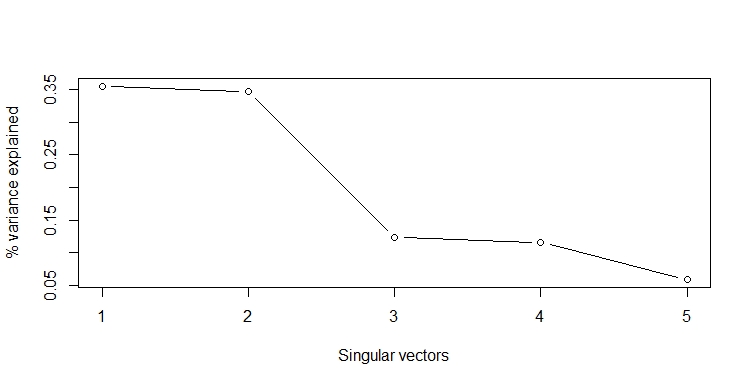
The first two singular vectors explain most of the variance. We could drop the last three without losing much information. However, when we look at the energy, we should retain 3 singular vectors

cumsum(s$d^2)/sum(s$d^2)
[1] 0.3552003 0.7020183 0.8254918 0.9410668 1.0000000

This shows that we can go from 171 columns (ncol(reviews_mat)) to 2, without loosing much information. LSI means that we should only keep the first 2 columns of: head(reviews_mat %*% s$v %*% solve(diag(s$d)))[,1:2].

To download the productreviews dataset click here¹.

Assume that:

• The tm package is loaded.