This exercise involves the Auto data set studied in the lab
(Here is the download link if you cannot find it anymore: Auto.csv ).
Make sure that the missing values have been removed from the data.
Auto <- read.csv("Auto.csv", header=T, na.strings="?")
Auto <- na.omit(Auto)
Earlier you saw how to index matrices, the same can be done on dataframes such as the Auto dataset.
class(Auto)
[1] "data.frame"
The apply() family pertains to the R base package and is populated with functions to manipulate slices of
data from matrices, arrays, lists and dataframes in a repetitive way.
These functions allow crossing the data in a number of ways and avoid explicit use of loop constructs.
The apply() functions form the basis of more complex combinations and help to perform operations with very few lines of code.
More specifically, the family is made up of the apply(), lapply() , sapply(), vapply(), mapply(), rapply(), and tapply() functions.
You can explore this family of functions.
For now, let us focus on sapply().
If we want to know the range of a quantitative variable, it is possible to use the range() function.
range(Auto$mpg)
[1]  9.0 46.6
If we want to know the range of every quantitative variable dataset, it possible to use the range()
function in conjunction with sapply().
We can select all the quantitative predictors by the following code: Auto[, 1:7].
sapply(Auto[, 1:7], range)

      mpg cylinders displacement horsepower weight acceleration year
[1,]  9.0         3           68         46   1613          8.0   70
[2,] 46.6         8          455        230   5140         24.8   82
The same can be done with other functions (e.g., mean() or sd())
Question
Some of the exercises are not tested by Dodona (for example the plots), but it is still useful to try them.
- What is the mean and standard deviation of each quantitative
predictor? (store them in
Auto.meanandAuto.sdrespectively) - Remove the 10th through 85th observations. What is the mean and standard deviation of each predictor in the
subset of the data that remains? (store them in
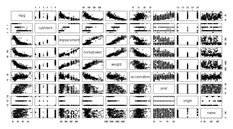
Auto.mean2andAuto.sd2respectively) - Using the full data set, investigate the predictors graphically, using scatterplots or other tools of your choice. Create some plots highlighting the relationships among the predictors.
An example of how these plots could look like:

- Suppose that we wish to predict gas mileage (
mpg) on the basis of other variables. Do your plots suggest that any of the other variables might be useful in predictingmpg?