Next we add details to modnn that control the fitting algorithm. Here we have simply followed the examples given in the Keras book. We minimize squared-error loss as in

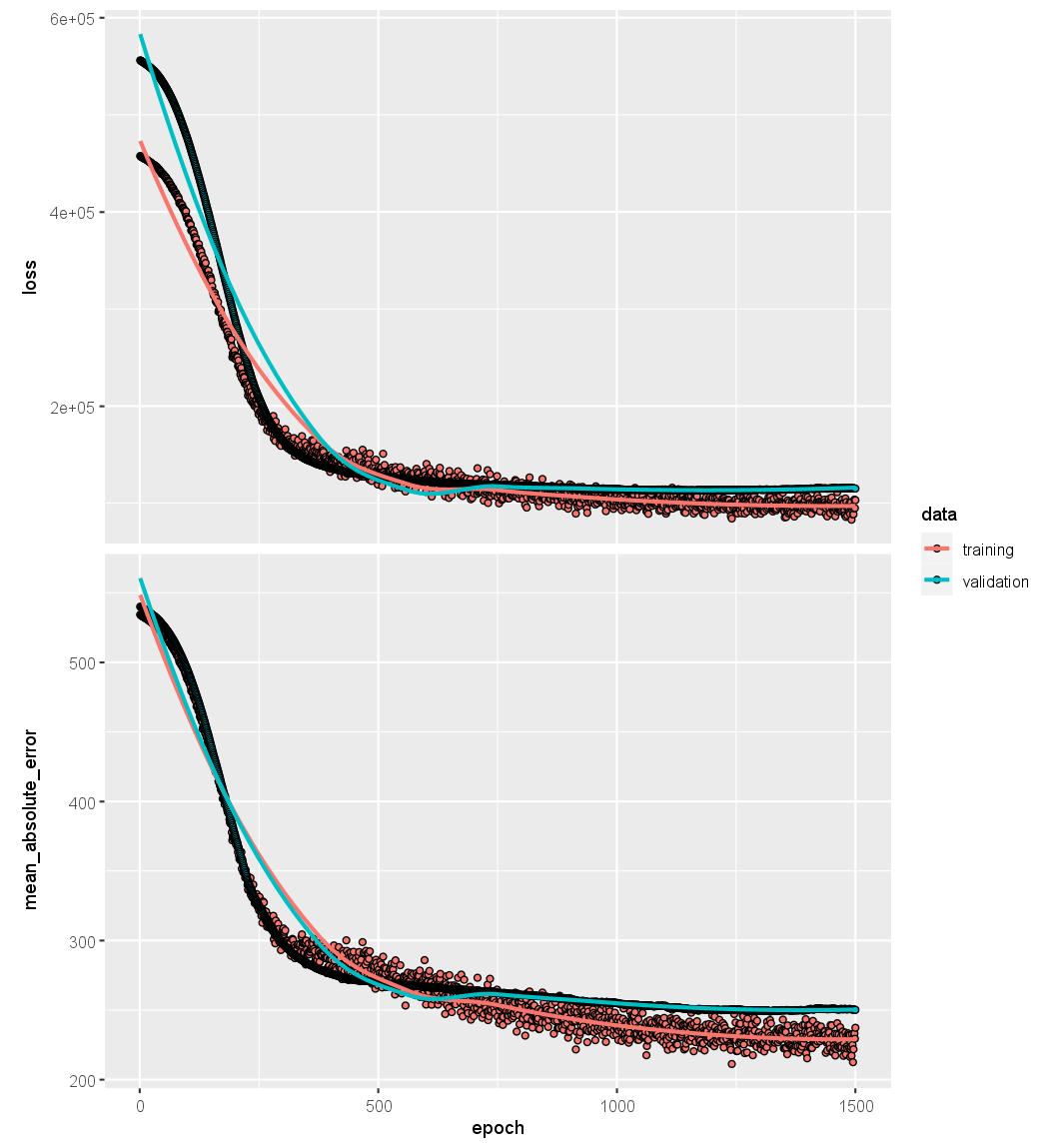
\[\underset{\left\{w_{k}\right\}_{1}^{K}, \beta}{\operatorname{minimize}} \frac{1}{2} \sum_{i=1}^{n}\left(y_{i}-f\left(x_{i}\right)\right)^{2}\]

The algorithm tracks the mean absolute error on the training data, and on validation data if it is supplied.

modnn %>% compile(loss = "mse",
                  optimizer = optimizer_rmsprop(),
                  metrics = list("mean_absolute_error"))

In the previous line, the pipe operator passes modnn as the first argument to compile(). The compile() function does not actually change the R object modnn, but it does communicate these specifications to the corresponding python instance of this model that has been created along the way.

Now we fit the model. We supply the training data and two fitting parameters, epochs and batch_size. Using 32 for the latter means that at each step of SGD, the algorithm randomly selects 32 training observations for the computation of the gradient. Recall from Sections 10.4 and 10.7 that an epoch amounts to the number of SGD steps required to process \(n\) observations. Since the training set has \(n = 176\), an epoch is \(176/32 = 5.5\) SGD steps. The fit() function has an argument validation_data; these data are not used in the fitting, but can be used to track the progress of the model (in this case reporting the mean absolute error). Here we actually supply the test data so we can see the mean absolute error of both the training data and test data as the epochs proceed. To see more options for fitting, use ?fit.keras.engine.training.Model.

history <- modnn %>% fit(
  x[-testid,], y[-testid], epochs = 1500, batch_size = 32,
  validation_data = list(x[testid,], y[testid]))

We can plot the history to display the mean absolute error for the training and test data. For the best aesthetics, install the ggplot2 package before calling the plot() function. If you have not installed ggplot2, then the code below will still run, but the plot will be less attractive.

plot(history)

plot

It is worth noting that if you run the fit() command a second time in the same R session, then the fitting process will pick up where it left off. Try re-running the fit() command, and then the plot() command, to see! Finally, we predict from the final model, and evaluate its performance on the test data. Due to the use of SGD, the results vary slightly with each fit. Unfortunately the set.seed() function does not ensure identical results (since the fitting is done in python), so your results will differ slightly.

npred <- predict(modnn, x[testid,])
mean(abs(y[testid] - npred))
[1] 250.1202

Questions

Compile the modnn model from the previous exercise as follows:
- Use the MSE as the loss function
- Use the optimizer_adam() as you optimizer
- Also track the mean_squared_error as a metric.
Fit the neural network on the training data for 1000 epochs and a batch size of 32. Supply the test data also as validation_data so you can monitor the train & test MSE. Store the result in history.
Visualize the loss and mean absolute error for the training and validation data in function of the number of epochs.
Store the predictions on the test data of the neural network in npred.
Store the MSE of the neural network on the test data in nmse.