RStudio will be our launching pad for data science projects. It not only provides an editor for us to create and edit our scripts but also provides many other useful tools. In this section, we go over some of the basics.
The panes
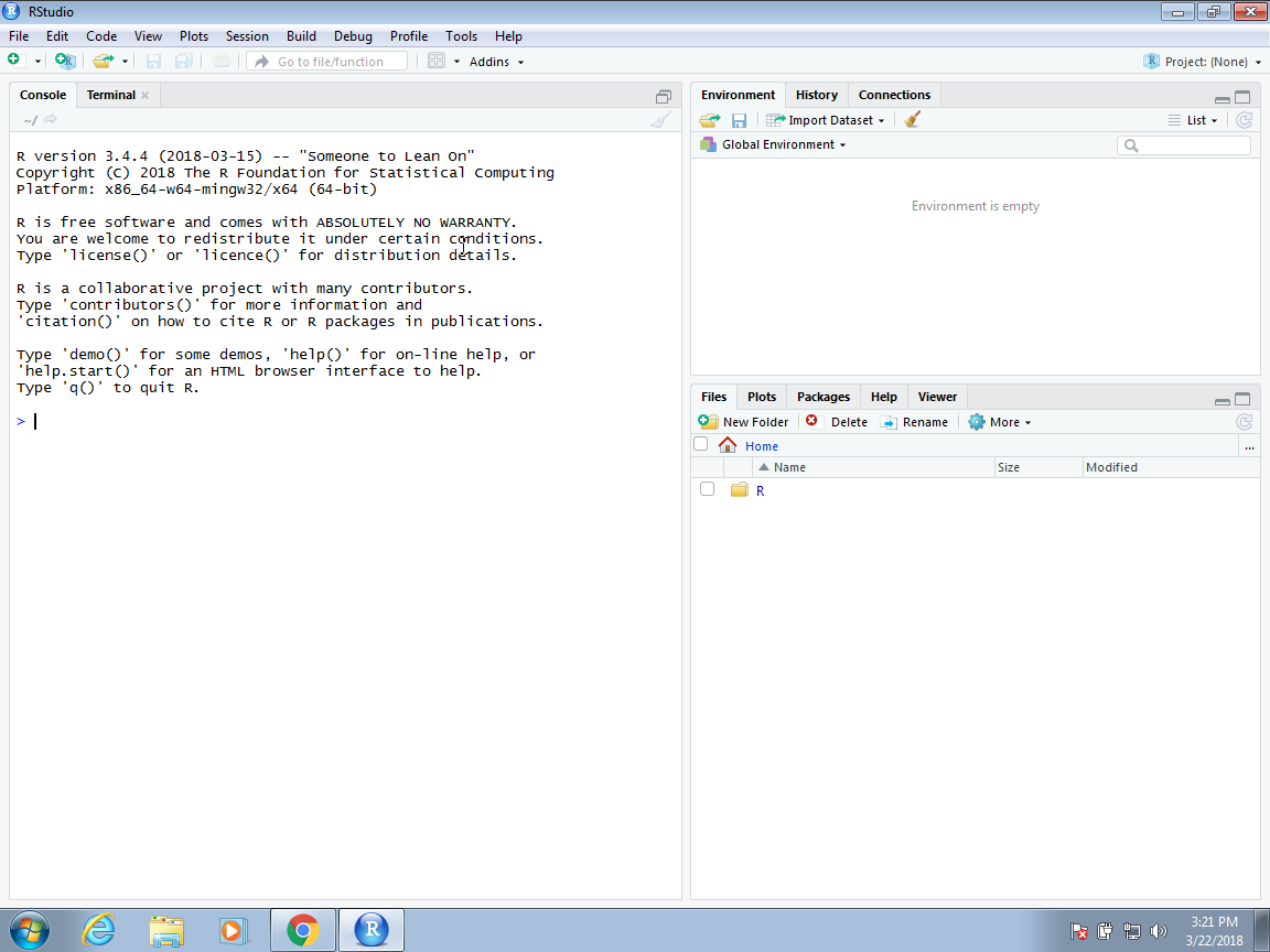
When you start RStudio for the first time, you will see three panes. The left pane shows the R console. On the right, the top pane includes tabs such as Environment and History, while the bottom pane shows five tabs: File, Plots, Packages, Help, and Viewer (these tabs may change in new versions). You can click on each tab to move across the different features.
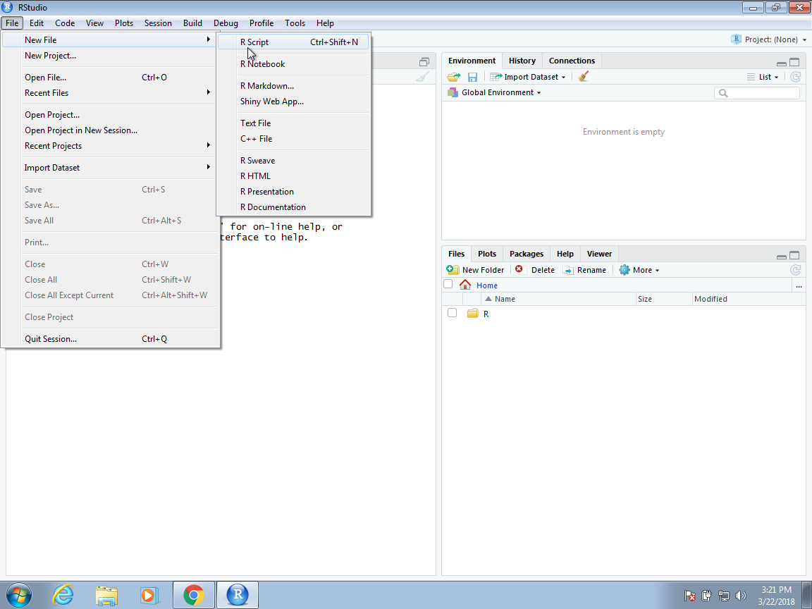
To start a new script, you can click on File, then New File, then R Script.
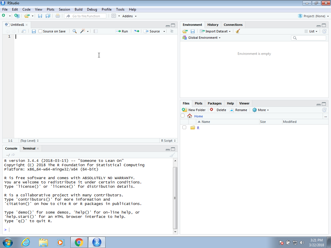
This starts a new pane on the left and it is here where you can start writing your script.
Key bindings
Many tasks we perform with the mouse can be achieved with a combination of key strokes instead. These keyboard versions for performing tasks are referred to as key bindings. For example, we just showed how to use the mouse to start a new script, but you can also use a key binding: Ctrl+Shift+N on Windows and command+shift+N on the Mac.
Although in this tutorial we often show how to use the mouse, we highly recommend that you memorize key bindings for the operations you use most. RStudio provides a useful cheat sheet with the most widely used commands. You can get it from RStudio directly:
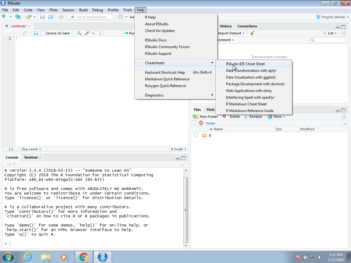
You might want to keep this handy so you can look up key-bindings when you find yourself performing repetitive point-and-clicking.
Running commands while editing scripts
There are many editors specifically made for coding. These are useful because color and indentation are automatically added to make code more readable. RStudio is one of these editors, and it was specifically developed for R. One of the main advantages provided by RStudio over other editors is that we can test our code easily as we edit our scripts. Below we show an example.
Let’s start by opening a new script as we did before. A next step is to
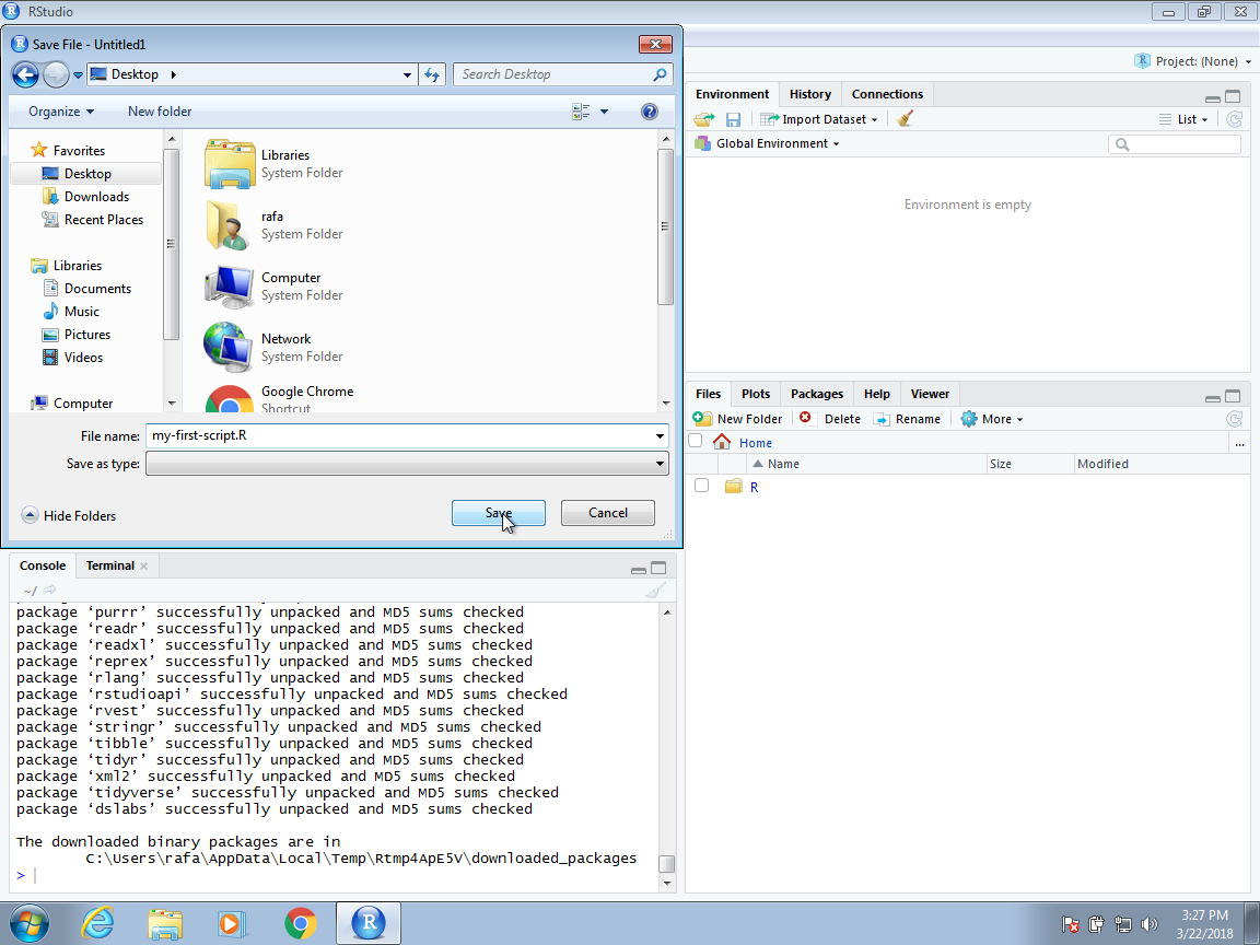
give the script a name. We can do this through the editor by saving the
current new unnamed script. To do this, click on the save icon or use
the key binding Ctrl+S on Windows and command+S on the Mac.
When you ask for the document to be saved for the first time, RStudio will prompt you for a name. A good convention is to use a descriptive name, with lower case letters, no spaces, only hyphens to separate words, and then followed by the suffix .R. We will call this script my-first-script.R.
Now we are ready to start editing our first script. The first lines of
code in an R script are dedicated to loading the libraries we will use.
Another useful RStudio feature is that once we type library() it
starts auto-completing with libraries that we have installed. Right now you have not installed any packages (see next chapter). If we would have installed tidyverse then RStudio will autocomplete if we type library(ti).
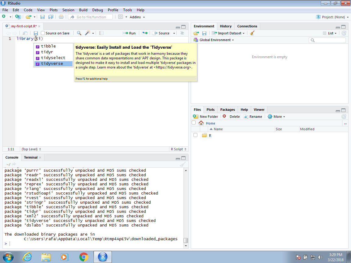
Another feature you may have noticed is that when you type library(
the second parenthesis is automatically added. This will help you avoid
one of the most common errors in coding: forgetting to close a
parenthesis.
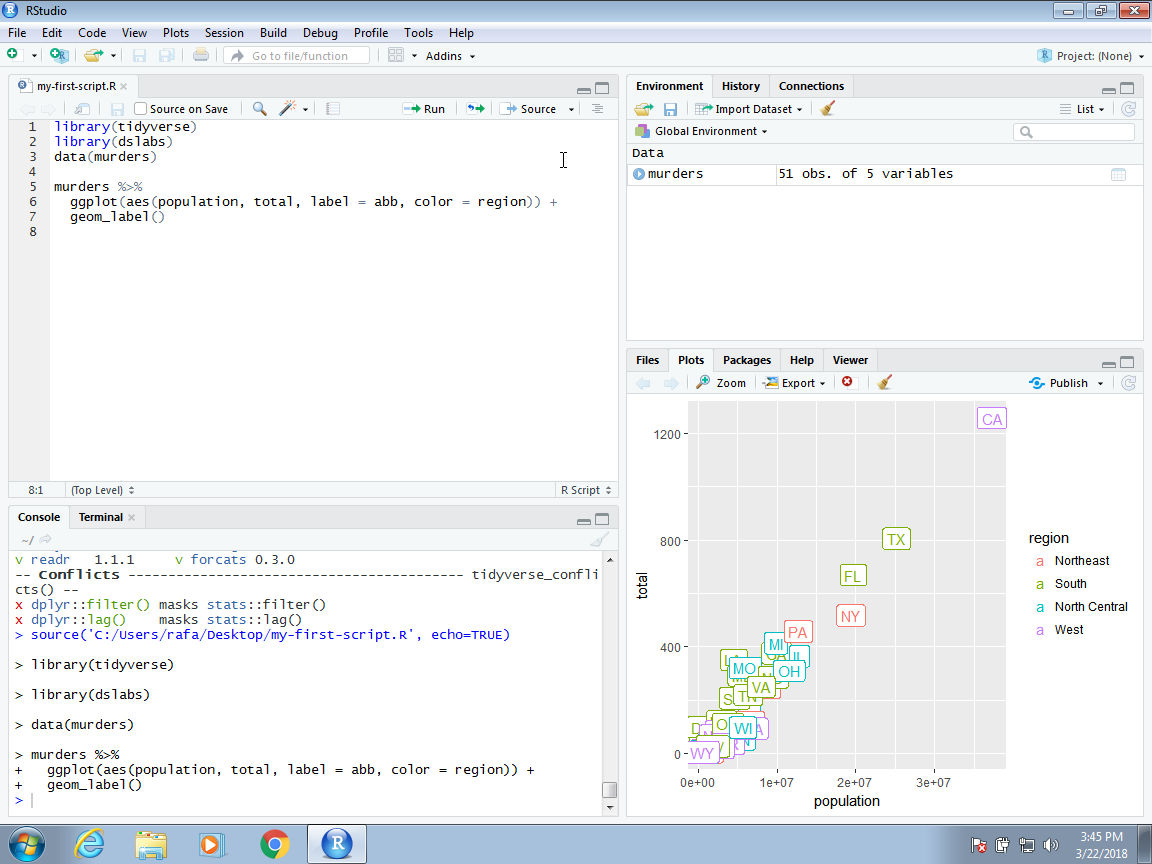
Now we can continue to write code. As an example, we will make a graph showing murder totals versus population totals by state. Once you are done writing the code needed to make this plot, you can try it out by executing the code. To do this, click on the Run button on the upper right side of the editing pane. You can also use the key binding: Ctrl+Shift+Enter on Windows or command+shift+return on the Mac.
Once you run the code, you will see it appear in the R console and, in this case, the generated plot appears in the plots console. Note that the plot console has a useful interface that permits you to click back and forward across different plots, zoom in to the plot, or save the plots as files.
To run one line at a time instead of the entire script, you can use Control-Enter on Windows and command-return on the Mac.
Changing global options
You can change the look and functionality of RStudio quite a bit.
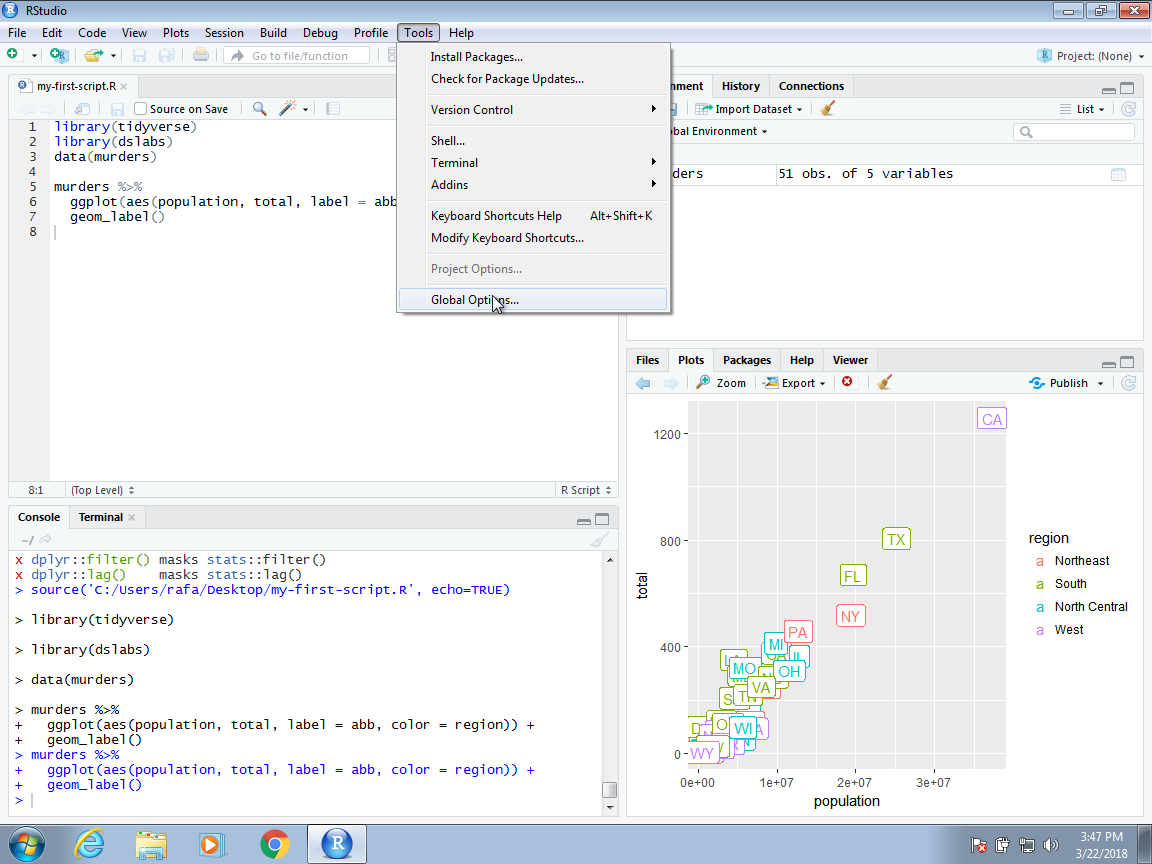
To change the global options you click on Tools then Global
Options…. <!–
As an example, we show how to change the appearance of the editor. To do this click on Appearance and then notice the Editor theme options.
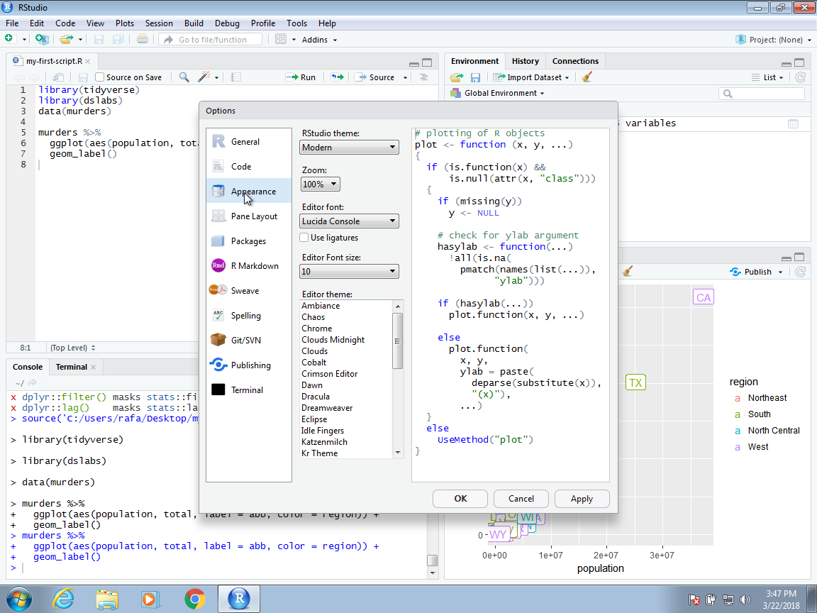
You can click on these and see examples of how your editor will look.
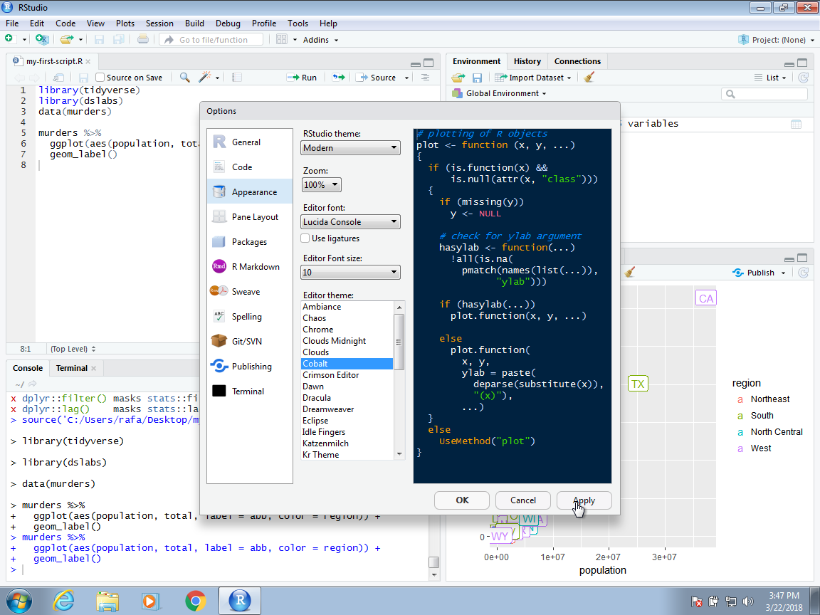
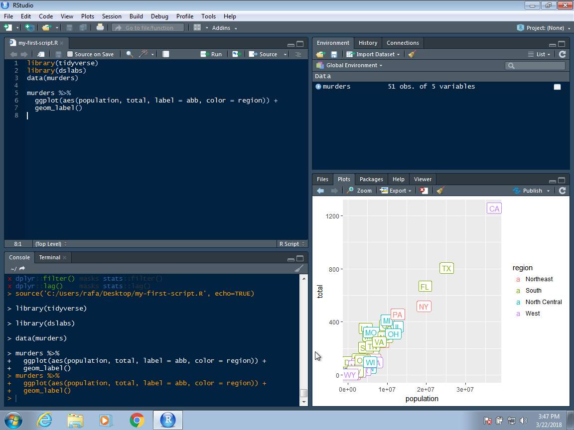
I personally like the Cobalt option. This makes your editor look like this:
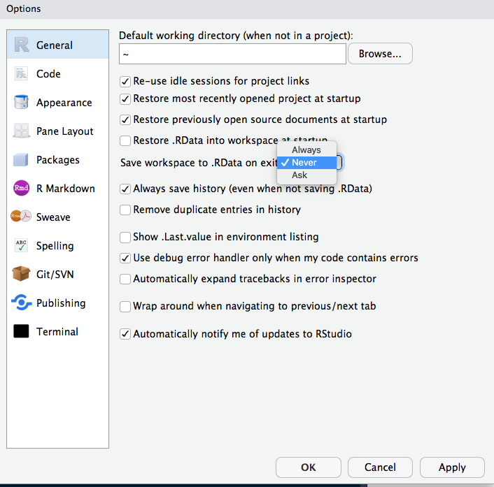
As an example we show how to make a change that we highly recommend. This is to change the Save workspace to .RData on exit to Never and uncheck the Restore .RData into workspace at start. By default, when you exit R saves all the objects you have created into a file called .RData. This is done so that when you restart the session in the same folder, it will load these objects. We find that this causes confusion especially when we share code with colleagues and assume they have this .RData file. To change these options, make your General settings look like this: