We can perform cross-validation using tune() to select the best choice of gamma and cost for an SVM with a radial kernel:

set.seed(1)
tune.out = tune(svm, y ~ ., data = dat[train,], kernel = "radial", ranges = list(cost = c(0.1, 1, 10, 100, 1000), gamma = c(0.5, 1, 2, 3, 4)))
summary(tune.out)

Parameter tuning of ‘svm’:
- sampling method: 10-fold cross validation 
- best parameters:
 cost gamma
    1   0.5
- best performance: 0.07 
- Detailed performance results:
    cost gamma error dispersion
1  1e-01   0.5  0.26 0.15776213
2  1e+00   0.5  0.07 0.08232726
3  1e+01   0.5  0.07 0.08232726
4  1e+02   0.5  0.14 0.15055453
5  1e+03   0.5  0.11 0.07378648
6  1e-01   1.0  0.22 0.16193277
7  1e+00   1.0  0.07 0.08232726
...

Therefore, the best choice of parameters involves cost=1 and gamma=0.5. We can view the test set predictions for this model by applying the predict() function to the data. Notice that to do this we subset the dataframe dat using -train as an index set.

table(true = dat[-train, "y"], pred = predict(tune.out$best.model, newdata = dat[-train,]))

    pred
true  1  2
   1 67 10
   2  2 21

12% of test observations are misclassified by this SVM.

Questions

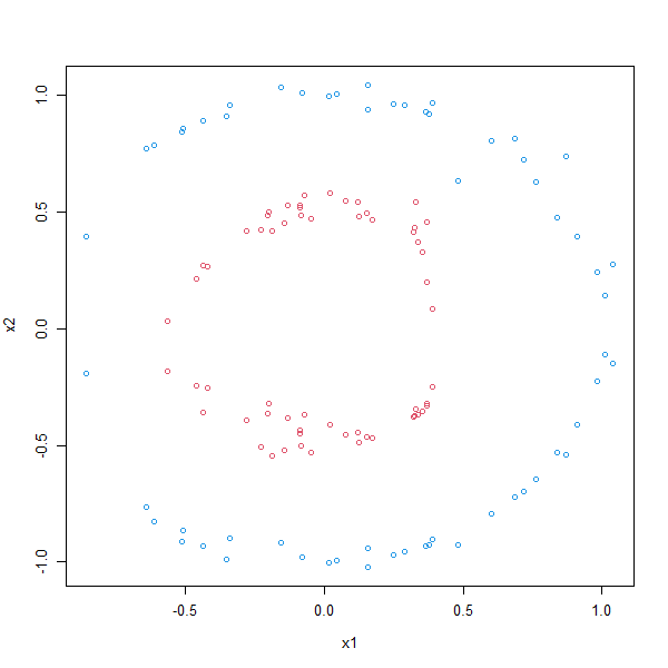
Different kernels can solve different problems. In this case we will try to solve a classification problem where the data is divided into a outer and inner circle:

make.circle.data = function(n) {
  x1 = runif(n, min = -1, max = 1)
  x2 = x1
  y1 = sqrt(1 - x1^2)
  y2 = (-1)*y1
  x1 = c(x1,x2)
  x2 = c(y1,y2)
  return(data.frame(x1, x2))
}

set.seed(2077)
df1 = make.circle.data(30)
df2 = make.circle.data(30)

df1 = df1 * .5 + rnorm(30, 0, 0.05)
df2 = df2 + rnorm(30, 0, 0.05)
df = rbind(df1, df2)
z = rep(c(-1, 1), each=60)

plot(df, col=z+3)

dat = data.frame(x=df, y = as.factor(z))
names(dat) = c('x.1', 'x.2', 'y')

• Split the dataframe dat into a train-validate set and a test set with a 80-20 split. Use the sample() function to randomly sample the data. Store the train-validate data in train and test data in test.
• Build three models each with a different kernel: linear, polynomial and radial. For each model:
  • Tune the model by performing ten-fold cross-validation and finding the best parameter value for cost in the range (0.01, 0.1, 1, 10, 100).
    • For the polynomial also find the best parameter value of degree in the range (2, 3, 4, 5).
    • For the radial also find the best parameter value of gamma in the range (0.5, 1, 2, 3, 4). Store the outcomes in lin.tune.out, poly.tune.out and rad.tune.out respectively
  • Predict the classes for the test data using the best model gotten from cross-validation. Store the predictions in lin.pred, poly.pred and rad.pred respectively.
• For each model look at the plot(BEST_MODEL, test) and answer the next multiple choice question

MC1: Which kernel is best able to solve the classification problem?
1) linear
2) polynomial
3) radial

---

Assume that:

• The e1071 library has been loaded