Now we use the cv.tree() function to see whether pruning the tree will improve performance.

set.seed(4)
cv.boston <- cv.tree(tree.boston)
plot(cv.boston$size, cv.boston$dev, type = 'b')

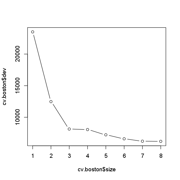
In this case, the most complex tree is selected by cross-validation. However, if we wish to prune the tree, we could do so as follows, using the prune.tree() function:

prune.boston <- prune.tree(tree.boston, best = 8)
plot(prune.boston)
text(prune.boston, pretty = 0) # same plot as previous exercise

In keeping with the cross-validation results, we use the unpruned tree to make predictions on the test set.

yhat <- predict(tree.boston, newdata = Boston[-train,])
boston.test <- Boston[-train, "medv"]
plot(yhat, boston.test)
abline(0, 1)
mean((yhat - boston.test)^2)
[1] 29.09147

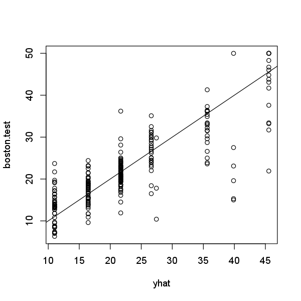
In other words, the test set MSE associated with the regression tree is 29.09. The square root of the MSE is therefore around 5.394, indicating that this model leads to test predictions that are within around $5,394 of the true median home value for the suburb.

Questions

• Below, you find a regression tree on the Hitters dataset, stored in the variable tree.hitters.
• Perform cross-validation to determine the optimal level of tree complexity. Use a seed value of 1. Store the model in the variable cv.hitters.
• Interpret the results and store the optimal number of nodes in the variable size.cv.
  (note: try to avoid hardcoding and use e.g. the which.min() function to find the index of the tree size with the lowest value for the dev attribute)
• MC1: will pruning increase the tree performance?
  • 1: No, CV selects the most complex tree
  • 2: Yes, CV selects a tree with 5 terminal nodes
  • 3: Yes, CV selects a tree with 7 terminal nodes
  • 4: Yes, CV selects a tree with 10 terminal nodes

Assume that:

• The ISLR2 and tree libraries has been loaded
• The Hitters dataset has been loaded and attached