For graph representation learning, we will mainly focus on node2vec because of its good performance and native R implementation. In order to make use of node2vec, the following package needs to be loaded first.

p_load(node2vec)

Introduction

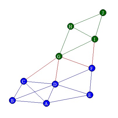
Let’s use the StudentNetwork data from the homophily exercise, because this had nice global and local characteristics and there were signs of homophily (you need homophily to make node2vec work). The resulting network looked as follows:

str(StudentsNetwork)
'data.frame':	19 obs. of  3 variables:
 $ from : chr  "A" "A" "A" "A" ...
 $ to   : chr  "B" "C" "D" "E" ...
 $ label: chr  "dd" "dd" "dd" "dd" ...

Node2vec

Node2vec uses the second order random walk with two parameter to guide the walk. Random walk is “second order”, that means in order to determine the next node it remembers the last node w and the second last node s_1. The return parameter p specifies the likelihood of immediately revisiting a node in the walk. A low p keeps the walk local to the starting node, hence resembling a breadth first search type of walk. A high value of p implies we are less likely to sample an already visited node in the next 2 steps. The in-out parameter q differentiates between inward and outward exploration of the nodes. If the value is less than 1, a depth first type of search is obtained. Vice-versa, if q is bigger than 1, a breadth first type of search is obtained. The in-out parameter q is also referred to as the walk-away parameter. Both p and q parameters allow our search procedure to interpolate between a breadth first and depth first strategy.

We calculate node2vec with the return parameter p equal to 1 and the in-out parameter q also equal to 1.

emb <- node2vecR(StudentsNetwork[,-3], p=1,q=1,num_walks=5,walk_length=5,dim=5)

Let’s have a look at the corresponding embeddings.

str(emb)
num [1:10, 1:5] -0.8227 0.0416 -0.36 0.0883 -0.1127 ...
 - attr(*, "dimnames")=List of 2
  ..$ : chr [1:10] "J" "E" "H" "G" ...
  ..$ : NULL

As you can see there are 10 rows (i.e., the number of nodes) and 5 columns (i.e., embedding size). Note that the rows have changes, this will always be the case when re-running node2vec!

Add a rowname to the embedding matrix, to know which node we are talking about

emb_name <- data.frame(node = row.names(emb), emb)

Let’s calculate the cosine similarity between node G and all the other nodes.

cos_sim <- sim2(x = as.matrix(emb), y = as.matrix(emb[emb_name$node == "G",, drop = FALSE]), method = "cosine", norm = "l2")
head(sort(cos_sim[,1], decreasing = TRUE), 10)
          G           B           C           J           F           I           A           H           D           E 
 1.00000000  0.62287998  0.30562320  0.04094266 -0.16848073 -0.20215207 -0.24295774 -0.38645765 -0.46513821 -0.76433515 

This gives some strange results, maybe the parameters p and q were not well-suited for this problem. Therefore, other values for parameters p and q will be tested in a second case, where we decrease the value of p and increase the value of q. We do this because a low p keeps the walk local to the starting node and if q is bigger than 1, a breadth first type of search is obtained.

Assume that:

• The StudentsNetwork variable is given.
• The node2vec library has been loaded.
• A random seed is set.