In the example in the previous section, we knew that there really were two clusters because we generated the data. However, for real data, in general we do not know the true number of clusters. We could instead have performed K-means clustering on this example with \(K = 3\).
> set.seed(4)
> km.out <- kmeans(x, 3, nstart = 20)
> km.out
K-means clustering with 3 clusters of sizes 17, 23, 10

Cluster means:
        [,1]        [,2]
1  3.7789567 -4.56200798
2 -0.3820397 -0.08740753
3  2.3001545 -2.69622023

Clustering vector:
 [1] 1 3 1 3 1 1 1 3 1 3 1 3 1 3 1 3 1 1 1 1 1 3 1 1 1 2 2 2 2 2 2 2 2 2 2 2 2 2 2 2 2 2 2 3 2 3 2 2 2 2

Within cluster sum of squares by cluster:
[1] 25.74089 52.67700 19.56137
 (between_SS / total_SS =  79.3 %)

Available components:

[1] "cluster"      "centers"      "totss"        "withinss"     "tot.withinss" "betweenss"    "size"         "iter"
[9] "ifault"
> plot(x, col = (km.out$cluster + 1), main = "K-Means Clustering Results with K=3", xlab = "", ylab = "", pch = 20, cex = 2)
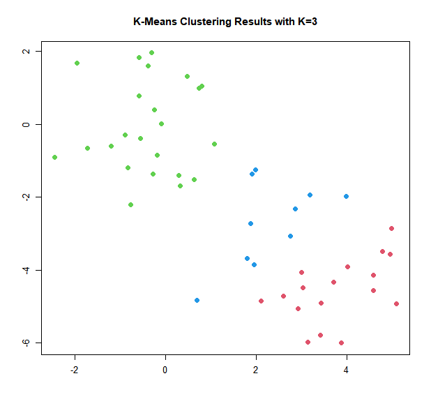
When \(K = 3\), K-means clustering splits up the two clusters.
Have a look at the following data.
Perform K-means clustering on the following dataset with nstart = 20.
Choose the optimal value for \(K\) yourself, by plotting the data for example.