Here we apply bagging and random forests to the Boston data, using the
randomForest package in R. The exact results obtained in this section may
depend on the version of R and the version of the randomForest package
installed on your computer. Recall that bagging is simply a special case of
a random forest with \(m = p\). Therefore, the randomForest() function can
be used to perform both random forests and bagging. We perform bagging
as follows:
library(randomForest)
set.seed(1)
bag.boston <- randomForest(medv ~ ., data = Boston, subset = train, mtry = 13, importance = TRUE)
bag.boston

Call:
 randomForest(formula = medv ~ ., data = Boston, mtry = 13, importance = TRUE, subset = train)
               Type of random forest: regression
                     Number of trees: 500
No. of variables tried at each split: 13

          Mean of squared residuals: 11.39601
                    % Var explained: 85.17
The argument mtry=13 indicates that all 13 predictors should be considered
for each split of the tree—in other words, that bagging should be done. How
well does this bagged model perform on the test set?
yhat.bag <- predict(bag.boston, newdata = Boston[-train,])
plot(yhat.bag, boston.test)
abline(0, 1)
mean((yhat.bag - boston.test)^2)
[1] 23.59273
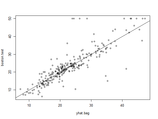
The test set MSE associated with the bagged regression tree is 23.59, which is significantly lower than the result obtained using an optimally-pruned single tree (29.09).
Questions
The mtcars data set contains information about fuel consumption (mpg) and 10 aspects of automobile design and performance for 32 cars.
In these exercises we will try to build a model that tries to predict the fuel consumption based on the automobile design and performance characteristics.
To gain more information about the data set you can type ?mtcars in your R console.
head(mtcars)
                   mpg cyl disp  hp drat    wt  qsec vs am gear carb
Mazda RX4         21.0   6  160 110 3.90 2.620 16.46  0  1    4    4
Mazda RX4 Wag     21.0   6  160 110 3.90 2.875 17.02  0  1    4    4
Datsun 710        22.8   4  108  93 3.85 2.320 18.61  1  1    4    1
Hornet 4 Drive    21.4   6  258 110 3.08 3.215 19.44  1  0    3    1
Hornet Sportabout 18.7   8  360 175 3.15 3.440 17.02  0  0    3    2
Valiant           18.1   6  225 105 2.76 3.460 20.22  1  0    3    1
- Sample the indices for the training set and store them in
train(70-30 split). - Train a bagging model on the training set with
mpgas the independent variable and all other variables as dependent variables. Store the model infit. - Make predictions on the test set. Store the predictions in
preds. - Calculate the MSE on the test set and store the result in
test.mse.
Assume that:
- The randomForest library has been loaded
- The mtcars data set has been loaded and attached