In order to fit a logistic regression GAM, we once again use the I() function in constructing the binary response variable, and set family=binomial.

gam.lr <- gam(I(wage > 250) ~ year + s(age, df = 5) + education, family = binomial, data = Wage)
par(mfrow = c(1, 3))
plot(gam.lr, se = T, col = "green")

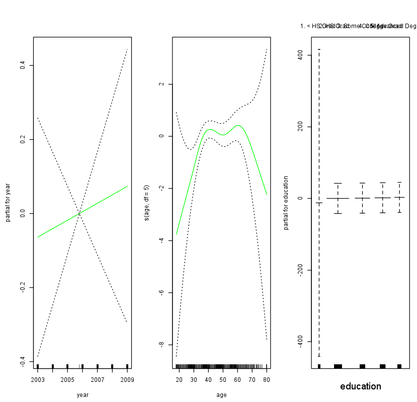
It is easy to see that there are no high earners in the <HS category:

table(education, I(wage > 250))

education            FALSE TRUE
  1. < HS Grad         268    0
  2. HS Grad           966    5
  3. Some College      643    7
  4. College Grad      663   22
  5. Advanced Degree   381   45

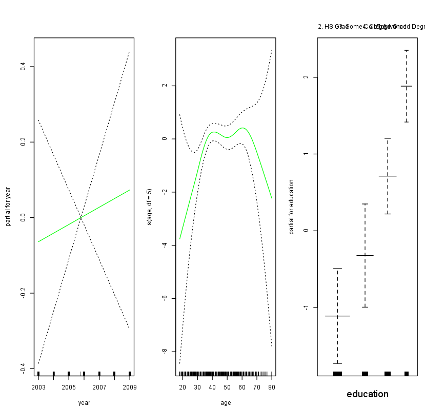
Hence, we fit a logistic regression GAM using all but this category. This provides more sensible results.

gam.lr.s <- gam(I(wage > 250) ~ year + s(age, df = 5) + education, family = binomial, data = Wage, 
                subset = (education != "1. < HS Grad"))
plot(gam.lr.s, se = T, col = "green")

Questions

• Create a GAM that predicts whether a neighbourhood has a median housing price larger than $ 30,000. Use the Boston dataset with medv as dependent variable and a smoothing spline of dis with 4 degrees of freedom as independent variable. Also include lstat as independent variable. Keep in mind that the median value medv is displayed in $1000s. Store the result in gam1.
• Calculate predictions for medv on the training set. Think about the type argument in the predict() function. Store the results in the variable preds.

Assume that:

• The MASS library has been loaded
• The Boston dataset has been loaded and attached