Social Network Learning: Quadratic Assignment Procedure (QAP) Regression

In this exercise, we will explore the Quadratic Assignment Procedure (QAP) Regression, a method used to test hypotheses about the relationships between network ties and nodal attributes. We will use the SharedTags and Gender data to illustrate this concept.

Setting Up

Before we begin, we need to set the working directory and load the data. The SharedTags and Gender data are read as follows:

setwd("...")
SharedTags <- read.csv("SharedTags.csv", header=FALSE)
Gender <- read.csv("Gender.csv", header=FALSE)

To explore the data, the function str() can be used. This will give us a glimpse of the structure of our data:

str(SharedTags, list.len=10)
str(Gender, list.len=10)

data.frame':	50 obs. of  50 variables:
 $ V1 : int  0 3 2 0 4 0 1 4 0 0 ...
 $ V2 : int  3 0 0 0 0 1 0 2 0 1 ...
 $ V3 : int  2 0 0 0 5 0 5 1 5 0 ...
 $ V4 : int  0 0 0 0 0 0 0 0 0 1 ...
 $ V5 : int  4 0 5 0 0 2 1 5 0 3 ...
 $ V6 : int  0 1 0 0 2 0 0 2 5 0 ...
 $ V7 : int  1 0 5 0 1 0 0 0 1 0 ...
 $ V8 : int  4 2 1 0 5 2 0 0 0 2 ...
 $ V9 : int  0 0 5 0 0 5 1 0 0 0 ...
 $ V10: int  0 1 0 1 3 0 0 2 0 0 ...
[list output truncated]

'data.frame':	50 obs. of  50 variables:
 $ V1 : int  1 0 0 0 1 0 0 1 0 0 ...
 $ V2 : int  0 1 0 0 1 1 0 1 0 1 ...
 $ V3 : int  0 0 1 1 1 1 0 0 1 0 ...
 $ V4 : int  0 0 1 1 0 1 1 0 0 0 ...
 $ V5 : int  1 1 1 0 1 1 0 1 1 1 ...
 $ V6 : int  0 1 1 1 1 1 0 1 0 0 ...
 $ V7 : int  0 0 0 1 0 0 1 0 0 0 ...
 $ V8 : int  1 1 0 0 1 1 0 1 0 1 ...
 $ V9 : int  0 0 1 0 1 0 0 0 1 1 ...
 $ V10: int  0 1 0 0 1 0 0 1 1 1 ...
[list output truncated]

The matrices are 50x50. The variable SharedTags is the response matrix. The question is if Gender explains SharedTags. The Gender matrix represents whether two persons have the same gender or not. The rows and columns represent persons.

QAP Regression

To start the analysis, the sna package is loaded.

if (!require(sna)){
  install.packages("sna",
                   repos="https://cran.rstudio.com/", 
                   quiet=TRUE)}
library(sna)

The QAP regression is performed using the netlm() function from the sna package. Before we can run the regression, we need to transform SharedTags and Gender to matrices, since these are data frames and sna requires matrices:

SharedTags <- as.matrix(SharedTags)
Gender <- as.matrix(Gender)

Next, Gender is transformed to a stack of independent network variables.

predictor_matrix <- array(NA, c(1, nrow(Gender), nrow(Gender))) 
predictor_matrix[1,,] <- Gender

This results in one row per predictor (i.e., 1), with the columns being the rows of the original matrix (n), and each layer representing a column of the original matrix (p). This is just the format that sna requires.

The function needed to do QAP regression is netlm() or netlogit() if the response is binary.

QAP_reg_mod <-netlm(y=SharedTags, 
                    x=predictor_matrix, 
                    test.statistic="beta")

The parameter test.statistic refers to whether an empirical distribution of beta or t-value is desired. Obviously t-values make more sense but for didactical purposes it is set to beta. Also a beta distribution is more flexible, so the most general and suited in a lot of cases.

The output can then be retrieved:

QAP_reg_mod <- summary(QAP_reg_mod)
QAP_reg_mod$names <- c("Intercept", "Gender")
QAP_reg_modThe

OLS Network Model

Residuals:
       0%       25%       50%       75%      100% 
-1.421227 -1.421227 -1.421222  1.578773  3.578778 

Coefficients:
          Estimate     Pr(<=b) Pr(>=b) Pr(>=|b|)
Intercept 1.421222e+00 1.000   0.000   0.000    
Gender    5.332395e-06 0.506   0.494   0.989    

Residual standard error: 1.778 on 2448 degrees of freedom
Multiple R-squared: 2.249e-12 	Adjusted R-squared: -0.0004085 
F-statistic: 5.506e-09 on 1 and 2448 degrees of freedom, p-value: 0.9999 


Test Diagnostics:

	Null Hypothesis: qap 
	Replications: 1000 
	Coefficient Distribution Summary:

        Intercept     Gender
Min     6.942e-01 -3.397e-01
1stQ    9.148e-01 -7.511e-02
Median  9.593e-01  5.332e-06
Mean    9.603e-01 -1.422e-03
3rdQ    1.003e+00  7.186e-02
Max     1.191e+00  2.940e-01

From this, we can conclude that Gender is not significant.

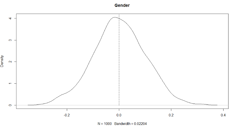
To have a visual idea, the empirical distributions for both the intercept and Gender are plotted as well as the coefficient (dashed line).

plot(density(QAP_reg_mod$dist[,1]), main='Intercept', xlim=c(0.65,1.5))
lines(rep(QAP_reg_mod$coefficients[1],2),c(0,6),lty=2)

plot(density(QAP_reg_mod$dist[,2]), main='Gender')
lines(rep(QAP_reg_mod$coefficients[2],2),c(0,6),lty=2)

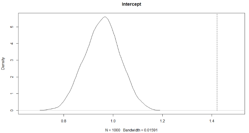
Since the intercept falls very much outside of the empirical distribution (i.e. it is an extreme value), it is significant. In other words, the chance that we will find a more extreme value is very small (0 in this case).

For the gender variable, the coefficient lays within the empirical distribution. This means that the coefficient most likely has the same distribution as the empirical. So, the coefficient is not significant.

OLS Network Model

Residuals:
        0%        25%        50%        75%       100% 
-0.4583333 -0.4583333 -0.2380952  0.5416667  0.7619048 

Coefficients:
          Estimate   Pr(<=b) Pr(>=b) Pr(>=|b|)
Intercept  0.4583333 0.910   0.090   0.090    
Gender    -0.2202381 0.085   0.956   0.184    

Residual standard error: 0.4712 on 88 degrees of freedom
Multiple R-squared: 0.05269 	Adjusted R-squared: 0.04192 
F-statistic: 4.894 on 1 and 88 degrees of freedom, p-value: 0.02954 

To download the gender dataframe click: here¹

To download the PadelNetwork click: here²

Assume that:

• The sna package has been loaded.
• The network package has been loaded.
• The adjacency_matrix for the PadelNetwork has been loaded.
• The dataframe gender has been loaded.