This exercise relates to the College data set, which can be found in
the ISLR library. It contains a number of variables for 777 different
universities and colleges in the US. The variables are
Private: Public/private indicatorApps: Number of applications receivedAccept: Number of applicants acceptedEnroll: Number of new students enrolledTop10perc: New students from top 10 % of high school classTop25perc: New students from top 25 % of high school classF.Undergrad: Number of full-time undergraduatesP.Undergrad: Number of part-time undergraduatesOutstate: Out-of-state tuitionRoom.Board: Room and board costsBooks: Estimated book costsPersonal: Estimated personal spendingPhD: Percent of faculty with Ph.D.’sTerminal: Percent of faculty with terminal degreeS.F.Ratio: Student/faculty ratioperc.alumni: Percent of alumni who donateExpend: Instructional expenditure per studentGrad.Rate: Graduation rate
Before reading the data into R, it can be viewed in Excel or a text editor.
Questions
Some of the exercises are not tested by Dodona (for example the plots), but it is still useful to try them.
- Use the
data(College)function to load in the data into R. - Look at the data using the
head()function. Try the following command:
head(college)
-
Use the
summary()function to produce a numerical summary of the variables in the data set. Store the summary insummary.num. -
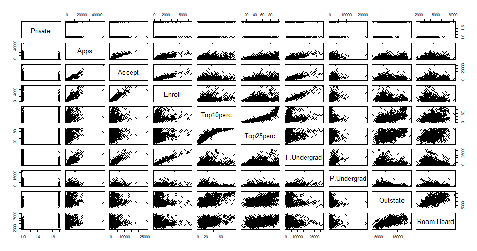
Use the
pairs()function to produce a scatterplot matrix of the first ten columns or variables of the data. Recall that you can reference the first ten columns of a matrixAusingA[,1:10].Your plot should look like this:
-
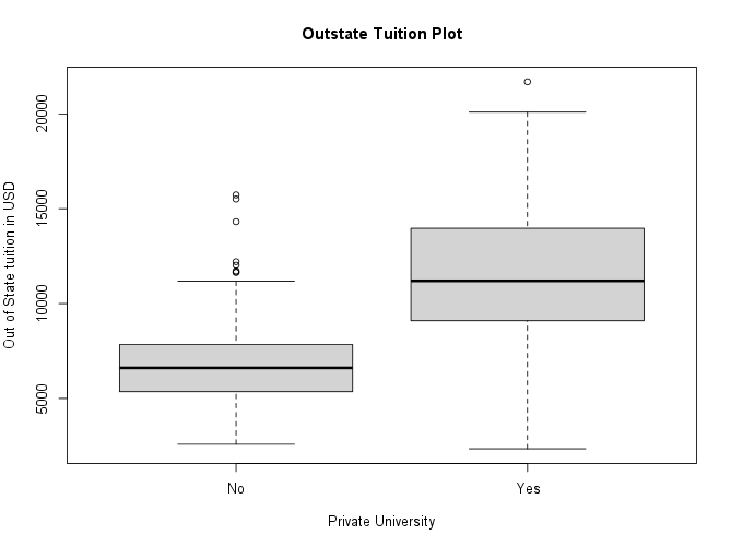
Use the
plot()function to produce side-by-side boxplots ofOutstateversusPrivate.Your plot should look like this:
-
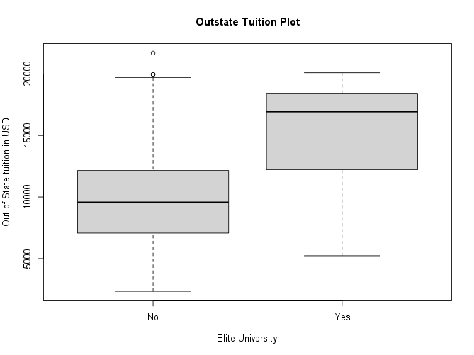
We create a new qualitative variable, called
Elite, by binning theTop10percvariable. We divide universities into two groups based on whether the proportion of students coming from the top 10% of their high school classes exceeds 50%.Elite <- rep("No", nrow(College)) Elite[College$Top10perc > 50] <- "Yes" Elite <- as.factor(Elite) College <- data.frame(College, Elite) -
Use the
summary()function to see how many elite universities there are. Store the summary in theelite.summaryvariable. Use the summary function only on theElitecolumn not the whole dataset -
Now use the
plot()function to produce side-by-side boxplots ofOutstateversusElite.Your plot should look like this:
-
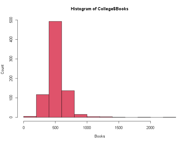
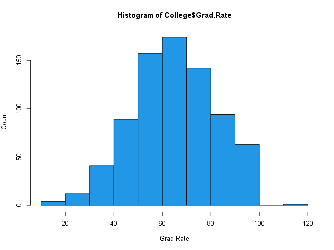
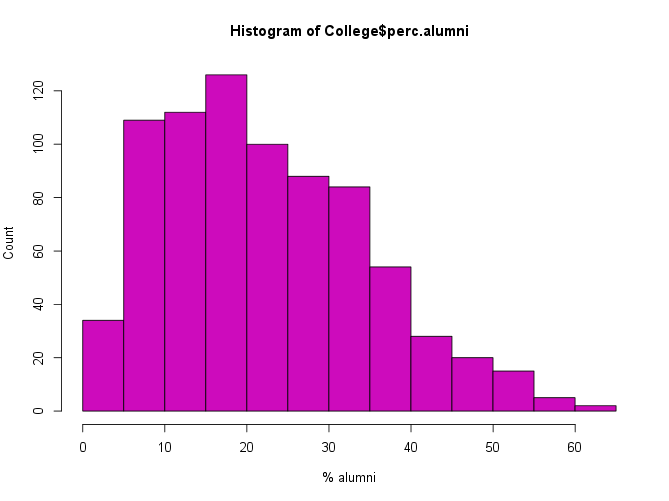
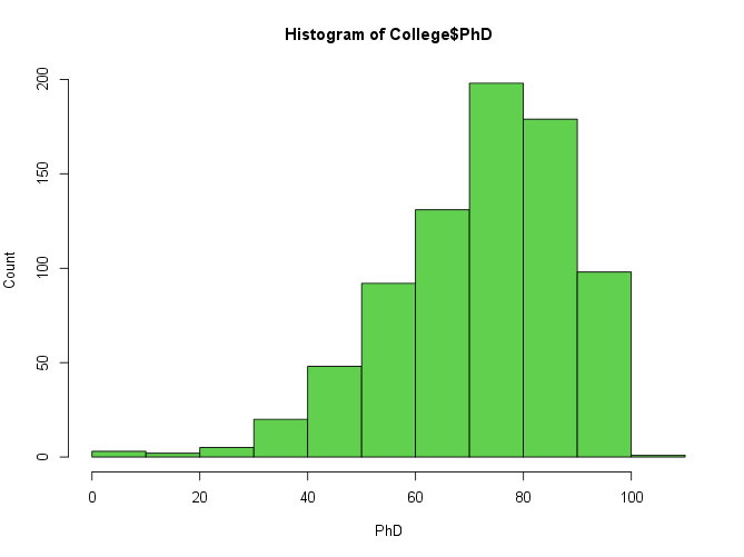
Use the
hist()function to produce some histograms with numbers of bins for a few of the quantitative variables.Your plots should look like this:
-
Continue exploring the data, and look for more interesting insights.
Assume that:
- The ISLR library has been loaded
- The College dataset has been loaded and attached