Random Forest Modeling

In this exercise, we will revisit the random forest algorithm in R. This algorithm should be familiar to you from the machine learning course. We will use the data_sets.Rdata to explain the random forest. The randomForest and AUC packages are required for this exercise.

Loading Required Packages and Data

if (!require("pacman")) install.packages("pacman"); require("pacman")
p_load(AUC, randomForest)

load("data_sets.Rdata")

Understanding the Data

The data contains information about a customer acquisition case. The independent variables are self-explanatory and contain the classical recency, frequency, and monetary value variables. The only variable that might be unclear is PaymentType_DD, which stands for the payment type direct debit.

str(BasetableTRAIN)

data.frame :	707 obs. of  7 variables:
 $ TotalDiscount          : num  129 0 19.3 0 0 ...
 $ TotalPrice             : num  130 951 870 964 962 ...
 $ TotalCredit            : num  0 0 0 -8.5 -6.18 ...
 $ PaymentType_DD         : num  0 0 0 0 0 0 0 0 0 0 ...
 $ PaymentStatus_Not.Paid : num  0 0 0 0 0 0 0 0 0 0 ...
 $ Frequency              : num  1 6 4 4 4 7 4 3 4 5 ...
 $ Recency                : num  243 310 216 141 8 58 55 345 372 319 ...

The dependent variable is acquisition in this case.

table(yTRAIN)

yTRAIN
0    1 
671  36

Building the Initial Random Forest Model

We can now create our first random forest model and make predictions.

rFmodel <- randomForest(
  x = BasetableTRAIN,
  y = yTRAIN,
  ntree = 1000,
  importance = TRUE
)
predrF <- predict(rFmodel, BasetableTEST, type = "prob")[, 2]
AUC::auc(roc(predrF, yTEST))

[1] 0.9226851

Tuning the Random Forest Model

To find the optimal value for ntree, we inspect the plotting curve. Note that you should add the validation set.

rFmodel <- randomForest(
  x = BasetableTRAIN,
  y = yTRAIN,
  xtest = BasetableVAL,
  ytest = yVAL,
  ntree = 1000,
  importance = TRUE
)
plot(rFmodel)

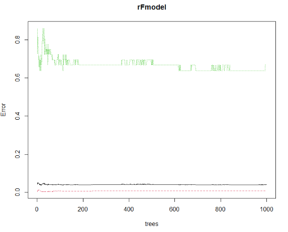
• Red dashed line : class error 0.
• Green dotted line : class error 1.
• Black solid line : OOB error.

It can be concluded that class 0 has a lower error than class 1. This is because there are much more zeros to learn from.

We can then create the model with the optimal ensemble size.

rFmodel <- randomForest(
  x = BasetableTRAINbig,
  y = yTRAINbig,
  ntree = which.min(rFmodel$test$err.rate[, 1]),
  importance = TRUE
)
predrF <- predict(rFmodel, BasetableTEST, type = "prob")[, 2]
AUC::auc(roc(predrF, yTEST))

[1] 0.8334513

However, the final performance is not better in this case. In general, it is not a good idea to tune the number of trees. Just set it to a high number by default, for example 500 or 1000.

Tuning the Number of Random Predictors

The number of random predictors can be tuned by adjusting the mtry parameter. We can create a loop for the mtry parameter and set the ntree to a high number.

m <- seq(1, ncol(BasetableTRAIN))
aucs <- numeric(length(m))

for (i in 1:length(m)) {
  print(i)
  rf <- randomForest(
    x = BasetableTRAIN,
    y = yTRAIN,
    ntree = 1000,
    mtry = m[i]
  )
  predrf <- predict(rf, BasetableVAL, type = 'prob')[, 2]
  aucs[i] <- AUC::auc(roc(predrf, yVAL))
}

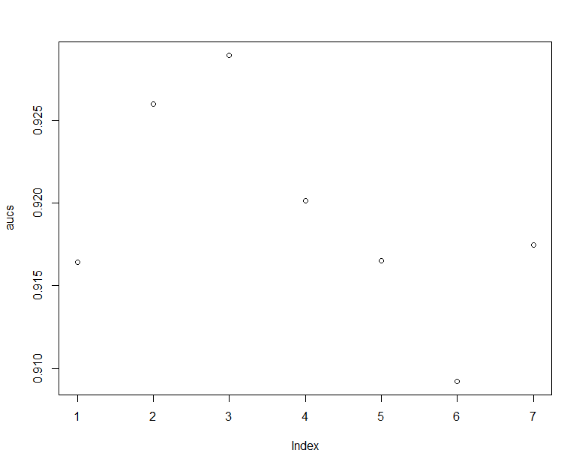
We can then find the optimal number of random predictors.

(mtry_opt <- which.max(aucs))

[1] 3

plot(aucs)

Building the Final Model

Finally, we can re-model with optimal parameters. Note that we are now using the big training set which combines train + validation.

rFmodel_opt <- randomForest(
  x = BasetableTRAINbig,
  y = yTRAINbig,
  ntree = 1000,
  mtry = mtry_opt,
  importance = TRUE
)
predrF_opt <- predict(rFmodel_opt, BasetableTEST, type = "prob")[, 2]
AUC::auc(roc(predrF_opt, yTEST))

[1] 0.9228818

To download the Covid-19 data click: here¹

Assume that:

• The AUC library has been loaded.
• The randomForest library has been loaded.
• The Covid-19 data has been loaded.