Recall from
\[\textnormal{FWER}(\alpha) = 1 - \prod_{j=1}^{m}(1 - \alpha) = 1 - (1 - \alpha)^m\]that if the null hypothesis is true for each of \(m\) independent hypothesis tests, then the FWER is equal to \(1-(1-\alpha)^m\). We can use this expression to compute the FWER for \(m = 1, \ldots , 500\) and \(\alpha = 0.05\), \(0.01\), and \(0.001\).
m <- 1:500
fwe1 <- 1 - (1 - 0.05)^m   # alpha = 0.05
fwe2 <- 1 - (1 - 0.01)^m   # alpha = 0.01
fwe3 <- 1 - (1 - 0.001)^m  # alpha = 0.001
We plot these three vectors in order to reproduce Figure 13.2. The red, blue, and green lines correspond to \(\alpha = 0.05\), \(0.01\), and \(0.001\), respectively.
par(mfrow = c(1, 1))
plot(m, fwe1, type = "l", log = "x", ylim = c(0, 1), col = 2,
     ylab = "Family - Wise Error Rate",
     xlab = "Number of Hypotheses")
lines(m, fwe2, col = 4)
lines(m, fwe3, col = 3)
abline(h = 0.05, lty = 2)
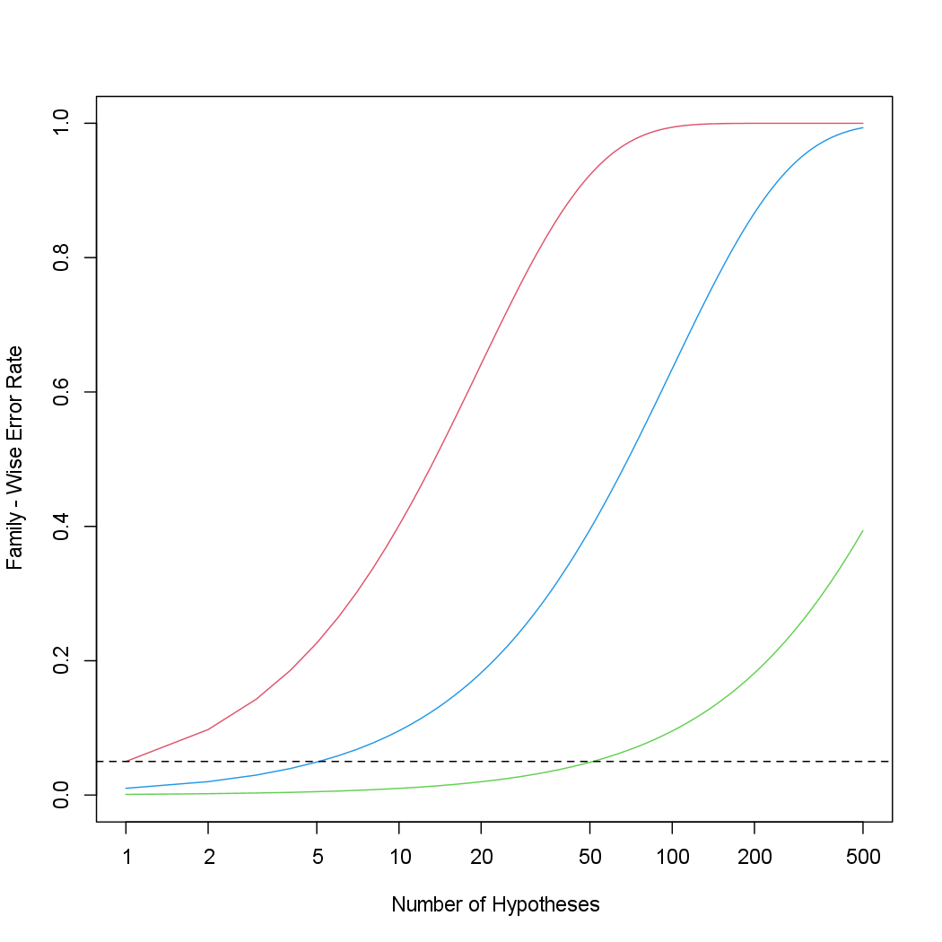
As discussed previously, even for moderate values of \(m\) such as \(50\), the FWER exceeds \(0.05\) unless \(\alpha\) is set to a very low value, such as \(0.001\). Of course, the problem with setting \(\alpha\) to such a low value is that we are likely to make a number of Type II errors: in other words, our power is very low.
We now conduct a one-sample t-test for each of the first five managers
in the Fund dataset, in order to test the null hypothesis that the \(j\)th fund
manager’s mean return equals zero, \(H_{0j}: μ_j = 0\).
> library(ISLR2)
> fund.mini <- Fund[, 1:5]
> t.test(fund.mini[, 1], mu = 0)
	One Sample t-test
data:  fund.mini[, 1]
t = 2.8604, df = 49, p-value = 0.006202
alternative hypothesis: true mean is not equal to 0
95 percent confidence interval:
 0.8923397 5.1076603
sample estimates:
mean of x
        3

> fund.pvalue <- rep(0, 5)
> for (i in 1:5)
+   fund.pvalue[i] <- t.test(fund.mini[, i], mu = 0)$p.value
> fund.pvalue
[1] 0.006202355 0.918271152 0.011600983 0.600539601 0.755781508
The p-values are low for Managers One and Three, and high for the other three managers. However, we cannot simply reject \(H_{01}\) and \(H_{03}\), since this would fail to account for the multiple testing that we have performed. Instead, we will conduct Bonferroni’s method and Holm’s method to control the FWER.
To do this, we use the p.adjust() function. Given the p-values, the function outputs
adjusted p-values, which can be thought of as a new set of
p-values that have been corrected for multiple testing. If the adjusted pvalue
for a given hypothesis is less than or equal to \(\alpha\), then that hypothesis
can be rejected while maintaining a FWER of no more than \(\alpha\). In other
words, the adjusted p-values resulting from the p.adjust() function can
simply be compared to the desired FWER in order to determine whether
or not to reject each hypothesis.
For example, in the case of Bonferroni’s method, the raw p-values are multiplied by the total number of hypotheses, \(m\), in order to obtain the adjusted p-values. (However, adjusted p-values are not allowed to exceed 1.)
> p.adjust(fund.pvalue, method = "bonferroni")
[1] 0.03101178 1.00000000 0.05800491 1.00000000 1.00000000
> pmin(fund.pvalue * 5, 1)
[1] 0.03101178 1.00000000 0.05800491 1.00000000 1.00000000
Therefore, using Bonferroni’s method, we are able to reject the null hypothesis only for Manager One while controlling the FWER at \(0.05\).
Questions
- Apply Holm’s Method by changing the
methodparameter to"holm". - MC1: Can we reject the null hypothesis that manager one and three at a FWER of \(0.05\)?
1) We can only reject the null hypothesis for manager one
2) We can only reject the null hypothesis for manager three
3) We can reject the null hypothesis for both manager one and three
4) We cannot reject the null hypothesis for manager one or three
Assume that:
- The
ISLR2library has been loaded - The
Funddataset has been loaded and attached