Numerical data that are not categorical also have distributions. In
general, when data is not categorical, reporting the frequency of each
entry is not an effective summary since most entries are unique. In our
case study, while several students reported a height of 68 inches, only
one student reported a height of 68.503937007874 inches and only one
student reported a height 68.8976377952756 inches. We assume that they
converted from 174 and 175 centimeters, respectively.
Statistics textbooks teach us that a more useful way to define a distribution for numeric data is to define a function that reports the proportion of the data below \(a\) for all possible values of \(a\). This function is called the cumulative distribution function (CDF). In statistics, the following notation is used:
\[F(a) = \mbox{Pr}(x \leq a)\]Here is a plot of \(F\) for the male height data:
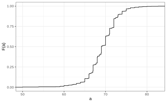
Similar to what the frequency table does for categorical data, the CDF defines the distribution for numerical data. From the plot, we can see that 16% of the values are below 65, since \(F(66)=\) 0.164, or that 84% of the values are below 72, since \(F(72)=\) 0.841, and so on. In fact, we can report the proportion of values between any two heights, say \(a\) and \(b\), by computing \(F(b) - F(a)\). This means that if we send this plot above to ET, he will have all the information needed to reconstruct the entire list. Paraphrasing the expression “a picture is worth a thousand words”, in this case, a picture is as informative as 812 numbers.
A final note: because CDFs can be defined mathematically the word empirical is added to make the distinction when data is used. We therefore use the term empirical CDF (eCDF).