We now fit a GAM to predict wage using natural spline functions of year and age, treating education as a qualitative predictor, as in equation

\[wage = \beta_0 + f_1(year) + f_2(age) + f_3(education) + \epsilon.\]

Since this is just a big linear regression model using an appropriate choice of basis functions, we can simply do this using the lm() function.

gam1 <- lm(wage ~ ns(year, 4) + ns(age, 5) + education, data = Wage)

We now fit the model in the equation above using smoothing splines rather than natural splines. In order to fit more general sorts of GAMs, using smoothing splines or other components that cannot be expressed in terms of basis functions and then fit using least squares regression, we will need to use the gam library in R. The s() function, which is part of the gam library, is used to indicate that we would like to use a smoothing spline. We specify that the function of year should have 4 degrees of freedom, and that the function of age will have 5 degrees of freedom. Since education is qualitative, we leave it as is, and it is converted into four dummy variables. We use the gam() function in order to fit a GAM using these components. All of the terms in the equation are fit simultaneously, taking each other into account to explain the response.

library(gam)
gam.m3 <- gam(wage ~ s(year, 4) + s(age, 5) + education, data = Wage)

In order to produce the figure below, we simply call the plot() function:

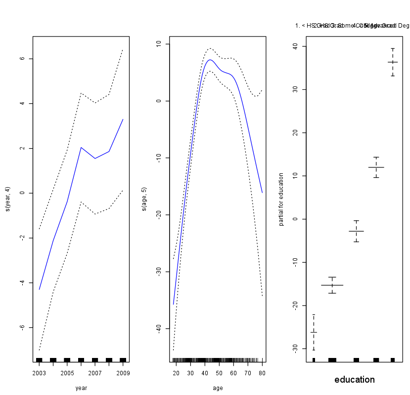
par(mfrow = c(1, 3))
plot(gam.m3, se = TRUE, col = "blue")

The generic plot() function recognizes that gam.m3 is an object of class gam, and invokes the appropriate plot.gam() method. Conveniently, even though gam1 is not of class gam but rather of class lm, we can still use plot.Gam() on it. The figure below was produced using the following expression:

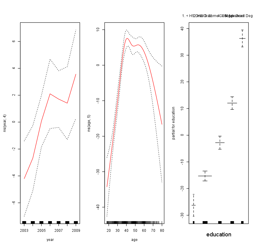
plot.Gam(gam1, se = TRUE, col = "red")

Notice here we had to use plot.Gam() rather than the generic plot() function.

Questions

• Fit a GAM on the Boston dataset to predict medv using a degree-3 regression spline of rm and a degree-4 natural spline of crim. Store the model in gam1.
• Fit a new model using smoothing splines, again degree-3 for rm and degree-4 for crim. Store the model in gam2.
• MC1: Invoke the plot.Gam() method of the class gam for both gam1 and gam2. Which command does not result in the appropriate plot? Try to understand why.
  • 1: plot.Gam(gam1)
  • 2: plot(gam1)
  • 3: plot.Gam(gam2)
  • 4: plot(gam2)

Assume that:

• The MASS library has been loaded
• The Boston dataset has been loaded and attached