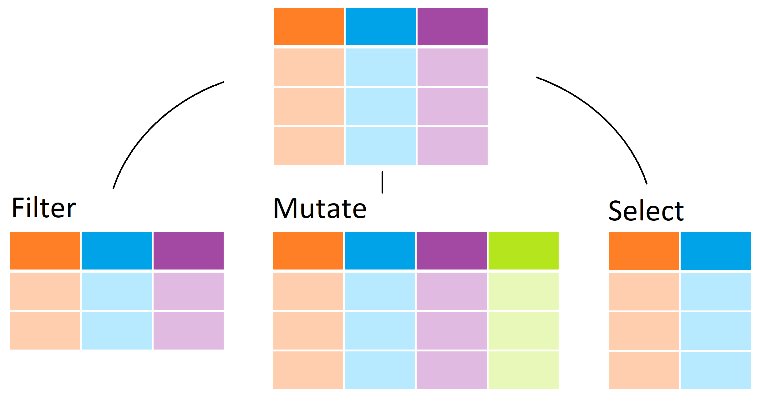
The dplyr package from the tidyverse introduces functions that perform some of the most common operations when working with data frames and uses names for these functions that are relatively easy to remember. For instance, to change the data table by adding a new column, we use mutate. To filter the data table to a subset of rows, we use filter. Finally, to subset the data by selecting specific columns, we use select.

Adding a column with mutate

We want all the necessary information for our analysis to be included in the data table. So the first task is to add the murder rates to our murders data frame. The function mutate takes the data frame as a first argument and the name and values of the variable as a second argument using the convention name = values. So, to add murder rates, we use:

library(dslabs)
data("murders")
murders <- mutate(murders, rate = total / population * 100000)

Notice that here we used total and population inside the function, which are objects that are not defined in our workspace. But why don’t we get an error?

This is one of dplyr’s main features. Functions in this package, such as mutate, know to look for variables in the data frame provided in the first argument. In the call to mutate above, total will have the values in murders$total. This approach makes the code much more readable.

We can see that the new column is added:

head(murders)
#>        state abb region population total rate
#> 1    Alabama  AL  South    4779736   135 2.82
#> 2     Alaska  AK   West     710231    19 2.68
#> 3    Arizona  AZ   West    6392017   232 3.63
#> 4   Arkansas  AR  South    2915918    93 3.19
#> 5 California  CA   West   37253956  1257 3.37
#> 6   Colorado  CO   West    5029196    65 1.29

Although we have overwritten the original murders object, this does not change the object that loaded with data(murders). If we load the murders data again, the original will overwrite our mutated version.

Subsetting with filter

Now suppose that we want to filter the data table to only show the entries for which the murder rate is lower than 0.71. To do this we use the filter function, which takes the data table as the first argument and then the conditional statement as the second. Like mutate, we can use the unquoted variable names from murders inside the function and it will know we mean the columns and not objects in the workspace.

filter(murders, rate <= 0.71)
#>           state abb        region population total  rate
#> 1        Hawaii  HI          West    1360301     7 0.515
#> 2          Iowa  IA North Central    3046355    21 0.689
#> 3 New Hampshire  NH     Northeast    1316470     5 0.380
#> 4  North Dakota  ND North Central     672591     4 0.595
#> 5       Vermont  VT     Northeast     625741     2 0.320

Selecting columns with select

Although our data table only has six columns, some data tables include hundreds. If we want to view just a few, we can use the dplyr select function. In the code below we select three columns, assign this to a new object and then filter the new object:

new_table <- select(murders, state, region, rate)
filter(new_table, rate <= 0.71)
#>           state        region  rate
#> 1        Hawaii          West 0.515
#> 2          Iowa North Central 0.689
#> 3 New Hampshire     Northeast 0.380
#> 4  North Dakota North Central 0.595
#> 5       Vermont     Northeast 0.320

In the call to select, the first argument murders is an object, but state, region, and rate are variable names.