Now we fit a model that makes use of additional predictors.
> fit.all <- coxph(Surv(time, status) ~ sex + diagnosis + loc + ki + gtv + stereo)
> fit.all
Call:
coxph(formula = Surv(time, status) ~ sex + diagnosis + loc +
    ki + gtv + stereo)

                       coef exp(coef) se(coef)      z        p
sexMale             0.18375   1.20171  0.36036  0.510  0.61012
diagnosisLG glioma  0.91502   2.49683  0.63816  1.434  0.15161
diagnosisHG glioma  2.15457   8.62414  0.45052  4.782 1.73e-06
diagnosisOther      0.88570   2.42467  0.65787  1.346  0.17821
locSupratentorial   0.44119   1.55456  0.70367  0.627  0.53066
ki                 -0.05496   0.94653  0.01831 -3.001  0.00269
gtv                 0.03429   1.03489  0.02233  1.536  0.12466
stereoSRT           0.17778   1.19456  0.60158  0.296  0.76760

Likelihood ratio test=41.37  on 8 df, p=1.776e-06
n= 87, number of events= 35
   (1 observation deleted due to missingness)
The diagnosis variable has been coded so that the baseline corresponds to
meningioma. The results indicate that the risk associated with HG glioma
is more than eight times (i.e. \(e^{2.15} = 8.62\)) the risk associated with meningioma.
In other words, after adjusting for the other predictors, patients
with HG glioma have much worse survival compared to those with meningioma.
In addition, larger values of the Karnofsky index, ki, are associated
with lower risk, i.e. longer survival.
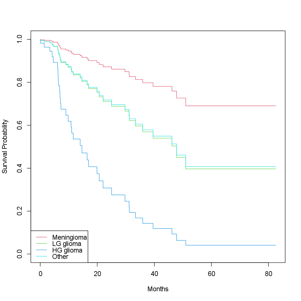
Finally, we plot survival curves for each diagnosis category, adjusting for
the other predictors. To make these plots, we set the values of the other
predictors equal to the mean for quantitative variables, and the modal value
for factors. We first create a data frame with four rows, one for each level
of diagnosis. The survfit() function will produce a curve for each of the
rows in this data frame, and one call to plot() will display them all in the
same plot.
modaldata <- data.frame(
  diagnosis = levels(diagnosis),
  sex = rep("Female", 4),
  loc = rep("Supratentorial", 4),
  ki = rep(mean(ki), 4),
  gtv = rep(mean(gtv), 4),
  stereo = rep("SRT", 4)
)
survplots <- survfit(fit.all, newdata = modaldata)
plot(survplots, xlab = "Months", ylab = "Survival Probability", col = 2:5)
legend("bottomleft", levels(diagnosis), col = 2:5, lty = 1)
Questions
- On the
Publicationdataset, model time-to-publication using all available predictor variables (except themechvariable). Store the model infit.all. - MC1: Which statement is true?
- 1) The chance of publication of a study with a positive result is 1.77 times higher than the chance of publication of a study with a negative result at any point in time, holding all other covariates fixed.
- 2) The chance of publication of a study with a negative result is 1.77 times higher than the chance of publication of a study with a positive result at any point in time, holding all other covariates fixed.
- 3) The chance of publication of a study with a positive result is 5.87 times higher than the chance of publication of a study with a negative result at any point in time, holding all other covariates fixed.
- 4) The chance of publication of a study with a negative result is 5.87 times higher than the chance of publication of a study with a positive result at any point in time, holding all other covariates fixed.
- MC2: Which statement is true on the 95% significance level?
- 1) The trial involving multiple centers has a significant impact on the chance of publication.
- 2) The trial focussing on a clinical endpoint does not have a significant impact on the chance of publication.
- 3) The sample size for the trail has a significant impact on the chance of publication.
- 4) The budget of the trial has no significant impact on the chance of publication.