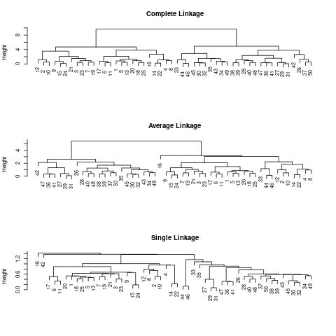
We can now plot the dendrograms obtained using the usual plot() function. The numbers at the bottom of the plot identify each observation.

par(mfrow = c(3, 1))
plot(hc.complete, main = "Complete Linkage", xlab = "", sub = "", cex = .9)
plot(hc.average, main = "Average Linkage", xlab = "", sub = "", cex = .9)
plot(hc.single, main = "Single Linkage", xlab = "", sub = "", cex = .9)

To determine the cluster labels for each observation associated with a given cut of the dendrogram, we can use the cutree() function:

cutree(hc.complete, 2)
 [1] 1 1 1 1 1 1 1 1 1 1 1 1 1 1 1 1 1 1 1 1 1 1 1 1 1 2 2 2 2 2 2 2 2 2 2 2 2 2 2 2 2 2 2 2 2 2 2 2 2 2
cutree(hc.average, 2)
 [1] 1 1 1 1 1 1 1 1 1 1 1 1 1 1 1 1 1 1 1 1 1 1 1 1 1 2 2 2 2 2 2 2 1 2 2 2 2 2 2 2 2 2 2 1 2 1 2 2 2 2
cutree(hc.single, 2)
 [1] 1 1 1 1 1 1 1 1 1 1 1 1 1 1 1 2 1 1 1 1 1 1 1 1 1 1 1 1 1 1 1 1 1 1 1 1 1 1 1 1 1 1 1 1 1 1 1 1 1 1

For this data, complete and average linkage generally separate the observations into their correct groups. However, single linkage identifies one point as belonging to its own cluster. A more sensible answer is obtained when four clusters are selected, although there are still two singletons.

cutree(hc.single, 4)
 [1] 1 1 1 1 1 1 1 1 1 1 1 1 1 1 1 2 1 1 1 1 1 1 1 1 1 3 3 3 3 3 3 3 3 3 3 3 3 3 3 3 3 4 3 3 3 3 3 3 3 3

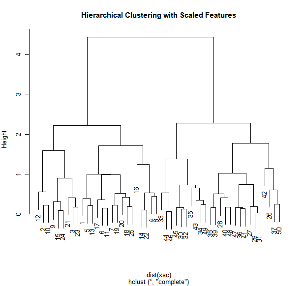
To scale the variables before performing hierarchical clustering of the observations, we use the scale() function:

par(mfrow = c(1, 1))
xsc <- scale(x)
plot(hclust(dist(xsc), method = "complete"), main = "Hierarchical Clustering with Scaled Features")

Questions

• Scale the data x, store the scaled data in xsc.
• Apply hierarchical clustering using single linkage on the scaled data and store the result in hc.single.
• Store the cluster labels associated with 4 cuts in hc.labels