In order to fit an SVM using a non-linear kernel, we once again use the svm()
function. However, now we use a different value of the parameter kernel.
To fit an SVM with a polynomial kernel we use kernel="polynomial", and
to fit an SVM with a radial kernel we use kernel="radial". In the former
case we also use the degree argument to specify a degree for the polynomial
kernel (this is d in \(K(x_i,x_{i'})=(1+\sum_{j=1}^{p}x_{ij}x_{i'j})^d\)), and in the latter case we use gamma to specify a
value of \(\gamma\) for the radial basis kernel \(K(x_i,x_{i'})=exp(-\gamma \sum_{j=1}^{p}(x_{ij}-x_{i'j})^2)\).
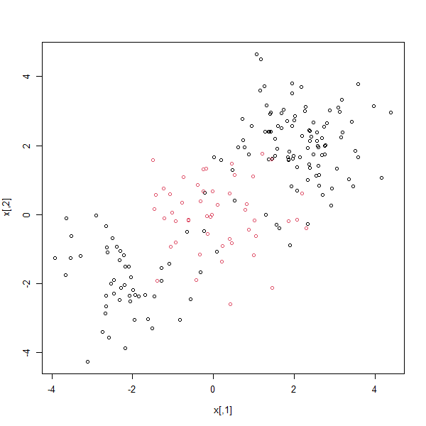
We first generate some data with a non-linear class boundary, as follows:
set.seed(1)
x <- matrix(rnorm(200 * 2), ncol = 2)
x[1:100,] <- x[1:100,] + 2
x[101:150,] <- x[101:150,] - 2
y <- c(rep(1, 150), rep(2, 50))
dat <- data.frame(x = x, y = as.factor(y))
Plotting the data makes it clear that the class boundary is indeed nonlinear:
plot(x, col = y)

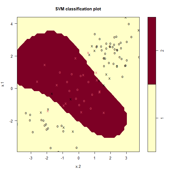
The data is randomly split into training and testing groups. We then fit
the training data using the svm() function with a radial kernel and \(\gamma = 1\):
train <- sample(200, 100)
svmfit <- svm(y ~ ., data = dat[train,], kernel = "radial", gamma = 1, cost = 1)
plot(svmfit, dat[train,])

The plot shows that the resulting SVM has a decidedly non-linear
boundary. The summary() function can be used to obtain some
information about the SVM fit:
summary(svmfit)

Call:
svm(formula = y ~ ., data = dat[train, ], kernel = "radial",
    gamma = 1, cost = 1)
Parameters:
   SVM-Type:  C-classification
 SVM-Kernel:  radial
       cost:  1
Number of Support Vectors:  31
 ( 16 15 )
Number of Classes:  2
Levels:
 1 2
Questions
- Create a model with a polynomial kernel with
degree = 3andcost = 1on the training data. Store the model insvmfit.
Assume that:
- The
e1071library has been loaded