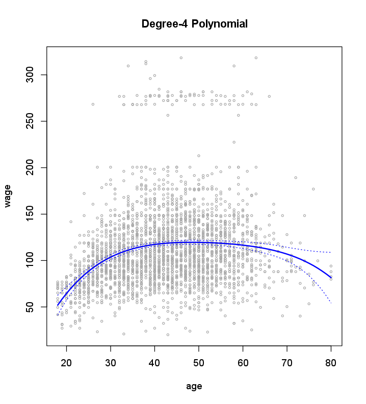
In this lab, we re-analyze the Wage data considered in the examples throughout this chapter, in order to illustrate the fact that many of the complex non-linear fitting procedures discussed can be easily implemented in R. We begin by loading the ISLR2 library, which contains the data.
library(ISLR2)
attach(Wage)
We now examine how the following figure is produced.

We first fit the model using the following command:
fit <- lm(wage ~ poly(age, 4), data = Wage)
coef(summary(fit))

                Estimate Std. Error    t value     Pr(>|t|)
(Intercept)    111.70361  0.7287409 153.283015 0.000000e+00
poly(age, 4)1  447.06785 39.9147851  11.200558 1.484604e-28
poly(age, 4)2 -478.31581 39.9147851 -11.983424 2.355831e-32
poly(age, 4)3  125.52169 39.9147851   3.144742 1.678622e-03
poly(age, 4)4  -77.91118 39.9147851  -1.951938 5.103865e-02
This syntax fits a linear model, using the lm() function, in order to predict
wage using a fourth-degree polynomial in age: poly(age,4). The poly() command
allows us to avoid having to write out a long formula with powers
of age. The function returns a matrix whose columns are a basis of orthogonal
polynomials, which essentially means that each column is a linear combination of the variables age, age^2, age^3 and age^4.
However, we can also use poly() to obtain age, age^2, age^3 and age^4
directly, if we prefer. We can do this by using the raw=TRUE argument to
the poly() function. Later we see that this does not affect the model in a
meaningful way—though the choice of basis clearly affects the coefficient
estimates, it does not affect the fitted values obtained.
fit2 <- lm(wage ~ poly(age, 4, raw = TRUE), data = Wage)
coef(summary(fit2))

                               Estimate   Std. Error   t value     Pr(>|t|)
(Intercept)               -1.841542e+02 6.004038e+01 -3.067172 0.0021802539
poly(age, 4, raw = TRUE)1  2.124552e+01 5.886748e+00  3.609042 0.0003123618
poly(age, 4, raw = TRUE)2 -5.638593e-01 2.061083e-01 -2.735743 0.0062606446
poly(age, 4, raw = TRUE)3  6.810688e-03 3.065931e-03  2.221409 0.0263977518
poly(age, 4, raw = TRUE)4 -3.203830e-05 1.641359e-05 -1.951938 0.0510386498
There are several other equivalent ways of fitting this model, which showcase
the flexibility of the formula language in R. For example
fit2a <- lm(wage ~ age + I(age^2) + I(age^3) + I(age^4), data = Wage)
coef(fit2a)

  (Intercept)           age      I(age^2)      I(age^3)      I(age^4)
-1.841542e+02  2.124552e+01 -5.638593e-01  6.810688e-03 -3.203830e-05
This simply creates the polynomial basis functions on the fly, taking care
to protect terms like age^2 via the wrapper function I() (the ^ symbol has
a special meaning in formulas).
fit2b <- lm(wage ~ cbind(age, age^2, age^3, age^4), data = Wage)
This does the same more compactly, using the cbind() function for building
a matrix from a collection of vectors; any function call such as cbind() inside
a formula also serves as a wrapper.
We now create a grid of values for age at which we want predictions, and
then call the generic predict() function, specifying that we want standard
errors as well.
agelims <- range(age)
age.grid <- seq(from = agelims[1], to = agelims[2])
preds <- predict(fit, newdata = list(age = age.grid), se = TRUE)
se.bands <- cbind(preds$fit + 2 * preds$se.fit, preds$fit - 2 * preds$se.fit)
Finally, we plot the data and add the fit from the degree-4 polynomial.
par(mfrow = c(1, 1))
plot(age, wage, xlim = agelims, cex = .5, col = "darkgrey")
title("Degree-4 Polynomial")
lines(age.grid, preds$fit, lwd = 2, col = "blue")
matlines(age.grid, se.bands, lwd = 1, col = "blue", lty = 3)
Questions
- Create a model with
wageas dependent variable using a third-degree polynomial inyear. Use the year variable directly and not the orthogonal polynomials. Store the model infit. - Calculate the predictions of
wagefor all values ofyear, ranging from the minimum to the maximum value ofyearin the dataset.
(note: we want all values in that range, not just the values present in the dataset). Store the results in variablepreds. - Calculate the confidence intervals (2 standard errors above and below the fit). Store the results in variable
se.bands.
Assume that:
- The ISLR2 library has been loaded
- The Wage dataset has been loaded and attached